Original citation:
Hobson, David and Klimmek, Martin (2012) Model-independent hedging strategies for
variance swaps. Finance and Stochastics, Vol.16 (No.4). pp. 611-649.
Permanent WRAP url:
http://wrap.warwick.ac.uk/50314
Copyright and reuse:
The Warwick Research Archive Portal (WRAP) makes the work of researchers of the
University of Warwick available open access under the following conditions. Copyright ©
and all moral rights to the version of the paper presented here belong to the individual
author(s) and/or other copyright owners. To the extent reasonable and practicable the
material made available in WRAP has been checked for eligibility before being made
available.
Copies of full items can be used for personal research or study, educational, or
not-for-profit purposes without prior permission or charge. Provided that the authors, title and
full bibliographic details are credited, a hyperlink and/or URL is given for the original
metadata page and the content is not changed in any way.
Publisher’s statement:
The original publication is available at
www.springerlink.com
A note on versions:
The version presented here may differ from the published version or, version of record, if
you wish to cite this item you are advised to consult the publisher’s version. Please see
the ‘permanent WRAP url’ above for details on accessing the published version and note
that access may require a subscription.
Model independent hedging strategies for variance swaps
David Hobson
Martin Klimmek
December 14, 2011
Abstract
A variance swap is a derivative with a path-dependent payoff which allows investors to take positions on the future variability of an asset. In the idealised setting of a continuously monitored variance swap written on an asset with continuous paths it is well known that the variance swap payoff can be replicated exactly using a portfolio of puts and calls and a dynamic position in the asset. This fact forms the basis of the VIX contract.
But what if we are in the more realistic setting where the contract is based on discrete monitoring, and the underlying asset may have jumps? We show that it is possible to derive model-independent, no-arbitrage bounds on the price of the variance swap, and corresponding sub- and super-replicating strategies. Further, we characterise the optimal bounds. The form of the hedges depends crucially on the kernel used to define the variance swap.
1
Introduction
The purpose of this article is to construct hedging strategies which super-replicate the payoff of a variance swap foranyprice path of the underlying asset, including price paths with jumps. The idea is that at initiation time 0, an agent purchases a portfolio of puts and calls which she holds until time
T. In addition, she follows a simple, dynamic investment strategy in the underlying over [0,T]. Then, for every possible path of the underlying, the sum of the payoff from the vanilla portfolio plus the gains from trade from the dynamic strategy is (more than) sufficient to cover the obligation from the variance swap. Implicit in this set-up is the idea that the super-hedge does not rely on any modelling assumptions. Instead, the super-hedge succeeds path-wise and is robust to the presence of jumps.
The problem of finding the cheapest super-hedging strategy can be seen as the dual of a primal problem which is to bound the prices for variance swaps over the class of all models for the asset price process which are consistent with the traded prices of puts and calls. If the variance swap is sold for the price upper-bound and hedged with the corresponding super-replicating strategy then the seller will not lose money under any scenario.
In addition to super-hedges and upper bounds on the price of the variance swap we also give sub-hedges and lower bounds. Moreover, our analysis is not restricted to any particular definition of the variance swap, nor is it based on a mathematical idealisation of a continuous time limit of the swap contract, but rather on a discrete set of observations. Nonetheless, the sub- and super-replicating hedges which work for discretely sampled variance swaps continue to work in the continuous time limit. As long as the price path has a quadratic variation, these limits exist by F ¨ollmer’s path-wise It ˆo formula [16].
This article shares the model-independent ethos for the pricing of variance swaps implicit in Neu-berger [24] and Dupire [15] in the setting of continuous price processes. In those articles, it was shown that if we assume that the asset price process is a continuous forward price, then the continuously monitored variance swap based on either squared log returns or squared simple returns is perfectly replicated by the following strategy: synthesise−2 log contracts using put and call options and trade
continuously in the asset to hold a number of shares equal to twice the reciprocal of the current asset price at all times. We will refer to this strategy as the classical continuous hedge. It follows that in the setting of a continuous forward price, the unique no-arbitrage price for the variance swap is equal to the price of the contract with payoffequal to−2 log contracts. This result holds independently of any
character, consisting of a static position in calls and puts and dynamic trading in the underlying. How-ever, the underlying setup is considerably more general, and the results more powerful since the hedges continue to super-replicate the variance swap for discontinuous price-paths and discrete monitoring over arbitrary time partitions. Nonetheless, this increase in generality comes at a cost in that instead of a replicating strategy we get sub- and super-replicating strategies and instead of a unique no-arbitrage price we get a no-arbitrage interval of prices.
As is well known, the model-independent analysis of derivative prices is related to the construction of extremal solutions for the Skorokhod embedding problem. This relationship was first developed in Hobson [17], see Hobson [18] for a recent survey, and exploits the idea that the classification of martingales with a given terminal law is equivalent to the classification of stopping times for Brownian motion, such that the stopped process has that given law. As we shall see, the monotone function which is associated with the cheapest super-hedging strategy arises in the Perkins solution [26] of the Skorokhod embedding problem [27]. For another example of model independent pricing and the connection between derivatives and the Skorokhod embedding problem in the context of variance options, see Cox and Wang [10]. In the setting of continuous price paths Cox and Wang [10] give bounds on the prices of call options on realised variance by exploiting a connection with the Root solution of the Skorokhod embedding problem.
In a recent paper [22], Kahal´e shows how to derive a tight sub-replicating strategy and corresponding model-independent lower bound for the price of a variance swap based on the squared log return kernel. The paper by Kahal´e was an inspiration for our study which grew from an attempt to relate his work to the previous literature on model-independent bounds and the Skorokhod embedding problem. By framing the problem in this way we extend the results of Kahal´e [22] to other kernels, and give upper bounds as well as lower bounds. Moreover, in the case of squared returns where the connection is particularly explicit, we explain the origin of the extremal models, and we give a natural interpretation for some of the quantities appearing in [22] in terms of the Perkins embedding of the Skorokhod embedding problem. The analysis of the squared returns kernel motivates our general approach to variance swap bounds and links this work to previous results of the authors (Hobson and Klimmek [19]) on characterising solutions of the Skorokhod embedding problem with particular optimality properties.
One of the features of our analysis is that we study the variance swap under a variety of definitions for the contract. Early definitions of the variance swap were based on squared simple daily returns. Accordingly, the first analysis of the discrepancy between the classical continuous hedge and realised variance in the presence of jumps, which is due to Demeterfi et. al. [12], focused on this kernel. Later, the finance industry switched to a standardised definition based on log-returns. (These contracts are typically sold OTC, and therefore any specification of the contract, and any observation frequency is possible.) In the presence of discrete monitoring or jumps (but not in the case of continuous monitoring and continuous price processes) each kernel lends different characteristics to variance swap values. Partly for this reason a variety of kernels have been proposed in the literature. Bondarenko [3] introduces a kernel which lies between the squared log return and squared simple return definitions. Bondarenko’s proposal is motivated by the fact that variance swaps based on this kernel can be replicated perfectly in the presence of jumps and in discrete time, see also Neuberger [25]. The kernel proposed by Carr and Corso [7] in the context of commodity markets, which is based on squared price differences, belongs to the same class. Recently Martin [23] has proposed yet another definition which is similar to the squared-return kernel but involves both the forward and the asset price. Our analysis covers all these kernels (though the kernel in [23] is only covered for the case of zero interest rates), and emphasises that the impact of jumps depends crucially on the nature of the kernel. We find that kernels split into two classes - below we name them increasing and decreasing kernels — and the special properties of the Bondarenko kernel come from the fact that it lies in the intersection of these classes.
raises fundamental questions about the validity of using the continuous time integrated variance as an approximation for the discretely monitored quantity. These previous studies underscore the importance of a model-independent analysis, especially one based on a finite number of monitoring points.
Recognising the importance of the jump contribution to variance swap values, Carr, Lee and Wu [9] show how it is possible to price and hedge a variance swap based on log returns if the asset price follows a L´evy model. The analysis is extended to a more general class of variation swaps in Carr and Lee [8]. Given a particular L´evy model for the dynamics of the price path, Carr and Lee show that there exists a model-dependent adjustment to the multiplier 2 appearing in the classical continuous hedge such that the value of the variance swap is given by the new multiplier times the price of a log-contract. In general, this price is not enforceable through a hedging strategy. Moreover, since all models are wrong and since the adjustment of the multiplier depends on specifying a particular model, this approach may still significantly mis-price realised variance, even if the L´evy model calibrates well to options prices.
The appeal of the classical continuous hedge of Neuberger and Dupire is that, apart from price-path continuity, the only necessary assumption is that a log contract can be synthesised from put and call options, and then the option payoff can be replicated perfectly along each path. In this article, we continue to assume that regular payoffs can be replicated with vanilla options, but relax the continuity assumption. The prices of variance swaps are highly sensitive to the presence of jumps, and so this is an important advance.
2
Main results
In this section we outline the main results of this article. Precise statements follow in the main body of the text, but here we describe the main theorems, and explain how they can be interpreted to give a model-independent bound on the price of a discretely monitored variance swap. Broadly speaking the results show firstly how to construct a family of model-independent sub-hedges for the variance swap (consisting of a static European position which may be synthesised with calls, and a simple dynamic trading position in the underlying) each of which is associated with a lower bound on the price of the variance swap; secondly how to choose the best (most expensive) strategy of this class; and thirdly that there are no other strategies of any class which outperform this best strategy without exposing the agent to model-risk. Fourthly we show how the results extend to super-hedges and upper bounds, and how they can be modified to cover other specifications of a variance swap.
Result 2.1. (See Theorem 5.10) Let f0,f1,...fNbe a sequence of positive real numbers.
(a) There exist a pair of functionsψ: (0,∞)→Randδ: (0,∞)→Rsuch thatψ(f0)=0and
N−1
X
k=0
fk+1−fk
fk !2
≥ψ(fN)+
N−1
X
k=0
δ(fk)(fk+1−fk). (1)
(b) There exists a family of such pairs of functions whereψ=ψκ,Ris given by
ψκ,R= (
ψκ,R(x) ψκ,R(z)
) =
2Rfx
0(x
−u)κ(u)u−3du x≥f0
ψκ,R(k(z))+ψ0κ,R(k(z))(z−k(z))+((z/k(z))−1)2 z<f0.
(2)
andδ=−ψ0
+, the right-derivative ofψ. Hereκis a decreasing functionκ: [f0,∞)7→(0,f0], and k is its
right-inverse. Note thatψis continuously differentiable on(f0,∞).
Result 2.2. (See Theorem 6.3) Letµbe a given probability measure on(0,∞)with mean f0and consider
sup κ
(Z
ψκ,R(f)µ(d f) )
where the supremum is taken over decreasing functionsκ: [f0,∞)7→(0,f0]. Then the supremum is attained by
Result 2.3. (See Theorem 7.7) Supposeµis as above and letψ=ψα(µ),R. Then there exists a stochastic model
(Ω,F,P,(Ft)0≤t≤T) supporting a stochastic process X=(Xt)0≤t≤T such that X0= f0, XT has law µ, X is a martingale, and
Z T
0 d[X]t
X2
t−
=ψ(XT)− Z T
0
ψ0
+(Xs−)dXs. (3)
The sequence f0,f1,...fN should be interpreted as the realised values of the forward price of an
asset evaluated on a grid of points 0=T0<T1< ... <TN=T. Then the payoffof the floating leg of a
discretely monitored variance swap (based on squared returns) isPN−1
k=0((fk+1−fk)/fk)2. Now consider a
trading strategy which involves holding a static position in European calls with payoffψ, coupled with a dynamic position in the forward wherebyδ(fk) units of the forward are held over the time-interval
(Tk,Tk+1] for eachk=0,1,...,N−1. The final payoffof such a strategy isψ(fN)+PN
−1
k=0 δ(fk)(fk+1−fk).
Then the inequality (1) above shows that it is possible to choose the pair (ψ,δ) such that the payoff of the variance swap dominates the terminal value of the trading strategy on a path-by-path basis. Consequently, no-arbitrage arguments give that the price of the variance swap is bounded below by the price of the European contract with payoffψ. (Note that the sumP
kδ(fk)(fk+1−fk) of forward contracts
is costless by definition.) The payoffψ≡ψ(fN) can be synthesised using calls, and if we assume that
calls with maturityTare traded, this contact can be priced in a model-independent fashion in terms of those traded calls. Hence, given the prices of call options, the first part of Result 2.1 can be used to give a model-independent bound on the price of a variance swap.
The second part of Result 2.1 gives a family of suitable hedging strategies, parameterised by a decreasing functionκ. Different choices of κwill lead to different lower bounds on the price of the variance swap. Given call prices, (or equivalently given the law of the forward price at time T as represented byµ) Result 2.2 shows how to choose the best contract based on functions (ψ,δ=−ψ0+)
of the given form by maximising the cost of the hedging portfolio, thus obtaining the best (highest) lower bound. Result 2.2 also relates the optimal contract to certain quantities which arise in the Perkins construction of the Skorokhod embedding problem.
Finally, Result 2.3 shows that the bounds we get from considering hedges of the given form are best possible, in the sense that in the case of continuous monitoring (or more generally in the limit as the partition becomes dense) there is a stochastic model for the forward price which is consistent with no-arbitrage and with the prices of traded calls and for which the payoffof the variance swap is equal, path-wise, to the payoffof the model-independent hedging strategy. Hence also, the model-based price of the variance swap is equal to the model-independent lower bound.
It is also possible to consider super-hedges and price upper bounds, and other definitions of the variance swap contract.
Result 2.4. (See Theorems 5.10, 6.3 and 7.7)
(a) There are analogous versions of Results 2.1, 2.2 and 2.3 for upper bounds for variance swaps based on the inequality
N−1
X
k=0
fk+1−fk
fk !2
≤ψ(fN)+
N−1
X
k=0
δ(fk)(fk+1−fk). (4)
This time the associated family of functions is based on a decreasing function`: (0,f0]7→[f0,∞), where the best choice of`is`=β(µ)where βis a quantity which arises in a ‘reversed’ Perkins solution of the Skorokhod embedding problem.
(b) There are analogous versions of Results 2.1, 2.2 and 2.3 for upper and lower bounds for variance swaps based on squared logarithmic returns, in which the left-hand-side of (1) or (4) is replaced byPN−1
k=0(logfk+1−
logfk)2, and the left-hand-side of (3) is replaced by[logX]T−[logX]0. Although the families of functions
(ψ,δ)change, they are again based on monotonic functions and the same functionsκ=α(µ)and`=β(µ)
yield the upper and lower bounds. However, for the squared logarithmic return payoffκ=α(µ)is now associated with the upper bound, and`=β(µ)is associated with the lower bound.
work to upper bounds and to other specifications of the variance swap. Kahal´e’s key contribution is to observe that an inequality of the form
(logy−logx)2≥ψ(y)−ψ(x)+δ(x)(y−x) (5)
can be summed along sequences (fk)0≤k≤Nto yieldPN −1
k=0(logfk+1−logfk)2≥ψ(fN)−ψ(f0)+PN
−1
k=0 δ(fk)(fk+1− fk) which is the analogue of (1). Hence in order to find lower bounds for the prices of variance swaps it
is sufficient to find solutions of (5).
Our primary goal in this paper is to prove theorems corresponding to the above results for a wide variety of definitions of the variance swap, including both squared returns and squared logarithmic returns. Our secondary goal is to explain why the model which is associated with the lower bound for squared log-return based contract is associated with the upper bound for the squared return contract and vice-versa (it turns out that the effect of jumps is opposite for these two contracts) and to explain why the optimal martingale is related to the Perkins solution of the Skorokhod embedding problem.
The remainder of the paper is structured as follows. In the next section we formally introduce the variance swap, and show how the definition depends on the form of the kernel. We also introduce the notions of model independent hedging, and consistent models. In Section 4 we study the problem in the setting of continuous monitoring for a process with jumps. We use this section to develop intuition and to explain why slightly different kernels can lead to opposite results. We also explain why for the squared return kernel the payoff of the variance swap is directly linked to a Skorokhod embedding problem.
The understanding we develop in Section 4 will motivate much of the subsequent analysis. Section 5 contains the first main theorem, and shows how to construct a class of sub-hedging strategies. In Sections 6 we find the most expensive sub-hedge of this class for a given set of call prices, and thus we derive a model independent bound on the price of a variance swap. Then in Section 7 we show this bound is best possible, by showing that in the continuous time limit it can be attained. Here we rely on F ¨ollmer’s work ([16]) on constructing It ˆo calculus without probability. In Section 8 we extend our results from contracts written on forwards to include the case of contracts written on undiscounted prices. The penultimate section gives some numerical results and in Section 10 we describe more precisely the contribution of this paper relative to the seminal paper by Kahal´e, [22].
3
Variance Swap Kernels and Model-Independent Hedging
3.1
Variation swaps
We begin by defining the payoffof a variance swap on a path-by-path basis. The payoffwill depend on a kernel, on the times at which the kernel is evaluated and on the asset price at these times.
Definition 3.1. (i) A variation swap kernel is a continuously differentiable bi-variate function H: (0,∞)×
(0,∞)→[0,∞)such that for all x∈(0,∞), H(x,x)=0=Hy(x,x). We say that the swap kernel is regular if
it is three times continuously differentiable.
A variance swap kernel is a regular variation swap kernel H such that Hyy(x,x)=x−2.
(ii) A partition P on[0,T]is a set of times0=t0<t1< ... <tN=T. A partition is uniform if tk=kTN, k=0,1,...N.
A sequence of partitionsP=(P(n))n≥1=({t(n)
k ; 0≤k≤N
(n)})
n≥1is dense iflim
n↑∞ sup
k∈{0,...,N(n)−1}
|t(n)
k+1−t (n)
k |=0.
(iii) A price realisation f =(f(t))0≤t≤Tis a c`adl`ag function f: [0,T]→(0,∞).
(iv) The payoffof a variation swap with kernel H for a partition P and a price realisation f is
VH(f,P)= N−1
X
k=0
H(f(tk),f(tk+1)). (6)
Remark 3.2. (i) Our main focus in this article is on variance swap kernels but we will discuss variation swap kernels HS(x,y)=(y−x)3 and HQ(x,y)=(y−x)2briefly, see Remark 4.1 and Example 7.10. (Strictly speaking HSis not a variation swap kernel since it is not non-negative, but most of our analysis still applies in this case.) A regular variation swap kernel is a variance swap kernel if H(x,x(1+δ))=δ2+o(δ2)for
δsmall. Examples of variance swap kernels include HR(x,y)=y−x
x 2
, HL(x,y)=(log(y)−log(x))2and HB(x,y)=−2log(y/x)−y−x
x
.
(ii) The price realisations f should be interpreted as realisations of the forward price of the asset with maturity T. Later we will extend the analysis to cover undiscounted price processes, rather than forward prices.
(iii) Large parts of the subsequent analysis can be extended to allow for price processes which can take the value zero, provided we also define H(0,0)=0, or equivalently truncate the sum in (6) at the first time in the partition that f hits 0. In this case we must have that zero is absorbing, so that if f(s)=0, then f(t)=0for all s≤t≤T.
(iv) In practice the variance swap contract is an exchange of the quantity V=VH(f,P)for a fixed amount K.
However, since there is no optionality to the contract, and since the contract paying K can trivially be priced and hedged, we concentrate solely on the floating leg.
(v) In many of the earliest academic papers, and in particular in Demeterfi et. al [12, 13], but also in some very recent papers, e.g. Zhu and Lian [28], the variance swap is defined in terms of the kernel HR. However, it has become market practice to trade variance swaps based on the kernel HL. Nonetheless these contracts are traded over-the-counter and in principle it is possible to agree any reasonable definition for the kernel. Variance swaps defined using the variance kernel HBwere introduced by Bondarenko [3], see
also Neuberger [25]. As we shall see, the contract based on this kernel has various desirable features. For continuous paths, in the limit of a dense partition the contract does not depend on the chosen kernel, see Example 7.10 and Lemma 7.9, but this is not the case in general.
(vi) The labels {S,Q,R,L,B} on the variation swap kernels denote {Skew, Quadratic, Returns, Logarithmic
returns, Bondarenko}respectively.
An important concept will be the quadratic variation of a path. For a dense sequence of partitionsP,
thequadratic variation[f] offonPis defined to be [f]t=limn↑∞P t(n)k ≤t(f(t
(n)
k+1)−f(t (n)
k ))
2, provided the limit
exists. We split the function into its continuous and discontinuous parts, [f]t=[f]ct+Pu≤t(∆f(u))2. Later
we will relate this definition to that introduced by F ¨ollmer [16], which is used to develop a path-wise version of It ˆo calculus. F ¨ollmer’s non-probabilistic It ˆo calculus has been used elsewhere in mathematical finance, most notably by Bick and Willinger [2], and helps emphasise the fact that the gains from trade have an interpretation as (the limit of) Riemann sums.
3.2
Model independent pricing
Our goal is to discuss how to price the variance swap contract, or more generally any path-dependent claim, under an assumption that European call and put (vanilla) options with maturityTare traded and can be used for hedging, but without any assumption that a proposed model is a true reflection of the real dynamics. In this sense the strategies and prices we derive are model independent.
Let call prices for maturity T be given by C(K), written as a function of strike and expressed in units of cash at time1 T. We assume that a continuum (in K) of calls are traded, and to preclude
arbitrage we assume that Cis a decreasing convex function such thatC(0)= f(0), C(K)≥(f(0)−K)+
and limK↑∞C(K)=0, see e.g. Davis and Hobson [11]. We exclude the case whereC(f(0))=0 for then C(K)=(f(0)−K)+ and the situation is degenerate: the forward price must remain constant and upper
and lower bounds on the price of the variance swap are zero. Although we assume that calls are traded today (time 0), we do not make any assumption on how call prices will behave over time, except that they will respect no-arbitrage conditions and that on expiry they will be worth the intrinsic value.
Definition 3.3. A synthesisable payoffis a functionψ: (0,∞)7→Rwhich can be represented as the difference of
two convex functions (so thatψ00
(x)exists as a measure).
Let Ψ ={ψ:ψ∈Ψ} be the set of synthesisable payoffs ψ: (0,∞)7→R. Then the left- and
right-derivativesψ0±(orψ 0
(x±)) exist and we have
ψ(f)=ψ(f(0))+ψ0(f(0)+)(f−f(0))+
Z
(0,f(0)]
(x−f)+ψ00(x)dx+
Z
(f(0),∞)
(f−x)+ψ00(x)dx. (7)
Thus we can represent the payoffof any sufficiently regular European contingent claim as a constant plus the gains from trade from holding a fixed quantity of forwards, plus the payoffof a static portfolio of vanilla calls and puts.
LetD[0,t] denote the space of c`adl`ag functions on [0,t].
Definition 3.4. A dynamic strategy for a fixed partition P is a collection of functions∆ =(δt0,...,δtN−1), where
δtj:D[0,tj]→R. The payoffof a dynamic strategy along a price realisation f is
N−1
X
k=0
δtk((f(t))0≤t≤tk)(f(tk+1)−f(tk)). (8)
Let∆¯(P)be the set of dynamic strategies.
Definition 3.5. ∆∈∆¯(P)is a Markov dynamic strategy ifδt
j(f(t)0≤t≤tj)=δtj(f(tj))for all j. A Markov dynamic strategy is a time homogeneous Markov dynamic strategy (THMD-strategy) ifδtj(f(tj))=δ(f(tj))for all j.
The quantityδtjrepresents the quantity of forwards to be held over the interval (tj,tj+1]. In principle
this quantity may depend on the current time and on the price history (f(t))0≤t≤tj. However, as we shall
see, for our purposes it is sufficient to work with a much simpler set of strategies where the quantity does not explicitly depend on time, nor on the price history except through the current value. We call this the Markov property, but note there are no probabilities involved here yet.
Definition 3.6. A semi-static hedging strategy(ψ,∆)is a functionψ∈Ψand a dynamic strategy∆∈∆¯(P). The
terminal payoffof a semi-static hedging strategy for a price realisation f is
ψ(f(T))+
N−1
X
k=0
δtk((f(t))0≤t≤tk)(f(tk+1)−f(tk)). (9)
Without loss of generality we may assume thatψ0(f(0)+)=0. If not then we simply adjust eachδtk
by the quantityψ0(f(0)+) and the payoffin (9) is unchanged. In the sequel, we will concentrate on the case when∆is a THMD strategy. Then we identify∆∈∆¯(P) withδ: (0,∞)→Rand write (ψ,δ) instead
of (ψ,∆).
Given that investments in the forward market may be assumed to be costless, the dynamic strategy has zero price. Thus, in order to define the price of a semi-static hedging strategy it is sufficient to focus on the price associated with the payofffunctionψ. The last two terms in (7) are expressed in terms of the payoffs of calls and puts. Thus we can identify the price ofψ(f(T)) with the price of a corresponding portfolio of vanilla objects. We also use put-call parity2to express the cost of the penultimate term in
(7) in terms of call prices. LetΨ0={ψ∈Ψ:ψ0+(f(0))=0}, and letΨc⊆Ψ0be the subset ofΨ0consisting
of the continuously differentiable functions.
Definition 3.7. The price of a semi-static hedging strategy(ψ∈Ψ0,∆∈∆¯(P))is
ψ(f(0))+
Z
(0,f(0)]
ψ00
(x)(C(x)−f(0)+x)dx+
Z
(f(0),∞)
ψ00
(x)C(x)dx.
The idea we wish to capture is that the agent holds a static position in calls together with a dynamic position in the underlying such that in combination they provide sub- and super-hedges for the claim.
2This means that we do not need to introduce a notation for the put price, which is convenient sincePis already in use for the partition. Put-call parity for the forward says that the price of a put with strikexis the price of a call with the same strike minus
Definition 3.8. Let G=G((f(tk))k=0,...N)be the payoffof a path-dependent option. Suppose that there exists a
semi-static hedging strategy(ψ,∆)such that on the partition P
G≤(respectively≥) ψ(f(T))+
N−1
X
k=0
δtk((f(t))0≤t≤tk)(f(tk+1)−f(tk)).
Then(ψ,∆)is called a semi-static super-hedge (respectively semi-static sub-hedge) for G.
Given a semi-static sub-hedge (respectively super-hedge) we say that the price of the sub-hedge (respectively super-hedge) is a model independent lower (respectively upper) bound on the price of the path-dependent claimG.
3.3
Consistent models
The aim of the agent is to construct a hedge which works path-wise, and does not depend on an underlying model. Nonetheless, sometimes it is convenient to introduce a probabilistic model and a stochastic process, and to interpret f(t) as a realisation of that stochastic process. In that case we work with a probability space (Ω,F,F=(Ft)0≤t≤T,P) supporting the stochastic processX=(Xt)0≤t≤T.
Definition 3.9. A model(Ω,F,F,P)and associated stochastic process X=(Xt)0≤t≤Tis consistent with the call prices(C(K))K≥0if(Xt)t≥0is a non-negative(F,P)-martingale and ifE[(XT−K)+]=C(K)for all K>0.
In the setting of a stochastic modelVH(X,P) :Ω→R+is a random variable, and forω∈Ω,VH(X(ω),P)
is a realised value of a variance swap. From a pricing perspective we are interested in getting upper and lower bounds onE[VH(X(ω),P)] as we range over consistent models. Knowledge of call prices is
equiv-alent to knowledge of the marginal law ofXTunder a consistent model (Breeden and Litzenberger [4]).
If we writeµfor the law ofXT and ifCµ(K)=E[(Zµ−K)+] where Zµ is a random variable with law
µ, then Xis consistent for the call pricesCif Cµ(K)=C(K). We writem=R0∞xµ(dx) and we assume, using the martingale property, thatX0=m. Then the problem of characterising consistent models is
equivalent to the problem of characterising all martingales with a given distribution at timeT.
4
Motivation
4.1
The continuous case
In the situation where both the monitoring and the price-realisations are continuous the theory for the pricing of variance swaps is complete and elegant. We will use this setting to develop intuition for the jump case.
Suppose that the price realisationfis continuous, and possesses a quadratic variation [f] : [0,T]→R+
on a dense sequence of partitionsP. Dupire [15] and Neuberger [24] independently made the observation
that the continuity assumption implies that a variance swap with payoffR0Tf(t)−2d[f]tcan be replicated
perfectly by holding a static portfolio of log contracts and trading dynamically in the underlying asset. Both Dupire and Neuberger assumef ≡Xis a realisation of a semi-martingale, but in our setting, the
observation follows from a path-wise application of It ˆo’s formula in the sense of F ¨ollmer [16], see Section 7. Applying It ˆo’s formula to−2 log(f(t)) we have
−2 log(f(T))+2 log(f(0))=−2
Z T
0
1
f(t)df(t)+
Z T
0
1
f(t)2d[f]t. (10)
Then, as we show in Section 7 below, down a dense sequence of partitionsVH(f,P∞)=limnVH(f,P(n))
exists and
VH(f,P∞)=
Z T
0
1
f(t)2d[f]t=−2 log(f(T))+2 log(f(0))+
Z T
0
2
f(t)df(t). (11)
payoff−2 log(f(T)/f(0)) and the gains from trade from a dynamic investment of 2/f(t) in the underlying.
Alternatively, the rightmost element of (11) can be viewed as the payoffof a semi-static hedging strategy in the continuous time limit for the choiceψ(x)=−2 log(x/f(0))+2(x−f(0))/f(0) and∆ =(δt)0≤t≤Twhere
δt((f(u))0≤u≤t)=(2/f(t))−(2/f(0)). Note that there is equality in (11) so that (ψ,δ) is both a sub- and
super-hedge forVH(f,P∞). In particular, under a price continuity assumption, the variance swap has a
model-independent price and an associated riskless hedge.
4.2
The e
ff
ect of jumps on hedging with the classical continuous hedge
Even if the continuity assumption cannot be justified, the associated replication strategy is nevertheless a reasonable candidate for a hedging strategy in the general case. Let us focus on the discrepancy between the payoffof the variance swap and the gains from trade resulting from using the hedge derived in the continuous case. The path-by-path It ˆo formula continues to apply in the case with jumps, see [16] and Section 7 below. Hence
−2 log(f(T))+2 log(f(0)) = −2
Z T
0
1
f(t−)df(t)+
Z T
0
1
f(t−)2d[f]
c t
+ X
0≤t≤T
2
( ∆
f(t)
f(t−)
!
−log 1+∆f(t)
f(t−)
!) .
Note thatd[log(f)]t=d[f]ct/f(t−)2+(∆log(f(t)))2. By adding and subtracting the discontinuous part of
the quadratic variation of log(f) on the right-hand-side of the above expression, we find
−2 log(f(T))+2 logf(0)=−2
Z T
0
1
f(t−)df(t)+[log(f)]T−
X
0≤t≤T
JL(∆f(t)/f(t−)) (12)
where
JL(η)=−2η+2 log(1+η)+log(1+η)2=−η3/3+O(η4).
It is intuitively clear, but see also Corollary 7.5, that VHL(f,P∞)≡[log(f)]T. Then it follows by
re-arrangement of equation (12) that the discrepancy between the realised value of the variance swap
VHL(f,P∞) and the return generated by the classical continuous hedging strategy can be represented as
the sum of the jump contributions:
VHL(f,P∞)− −2 log(f(T))+2 logf(0)+2
Z T
0
1
f(t−)df(t)
! = X
0≤t≤T JL ∆
f(t)
f(t−)
! .
We call this the hedging error with the convention that if the hedge sub-replicates the variance swap then the hedging error is positive.
Now consider the kernel HR and define V
HR(f,P∞)=
RT
0 d[f]t/f(t−)
2, again, see Corollary 7.5 for
justification. By a similar analysis (see also [12, 13]), but adding and subtracting∆f(ft(−t))
2
instead of the discontinuous part of the quadratic variation of log(f), we have
VHR(f,P∞)− −2 log(f(T))+2 log(f(0))+2
Z T
0
1
f(t−)df(t)
! = X
0≤t≤T JR
∆f(t)
f(t−)
! .
where
JR(η)=−2η+2 log(1+η)+η2=2η3/3+O(η4).
In the continuous case, under some mild regularity conditions onf andP, the variance swap value is
independent of the chosen kernel. In contrast, the value of a variance swap in the general case is highly dependent on the chosen kernel.
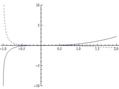
To see that this is the case, and to examine the impact of jumps on the hedging error for the kernelsHL
andHRwe consider the shapes of the functionsJ
RandJL, see Figure 1. For the kernelHL, a downward
classical continuous hedging strategy sub-replicatesVHL(f,P∞). Conversely, upward jumps result in a
[image:11.595.199.397.105.253.2]negative contribution to the hedging error. The story is reversed for the kernelHR.
Figure 1: JL(as represented by the dashed line) is convex decreasing forx≤0 and concave decreasing
forx≥0. In contrastJR(solid line) is first concave increasing and then convex increasing. The different
shapes of these two curves explains the different nature of the dependence of the payoffof the variance swap on upward and downward jumps for different kernels.
It follows from the argument in the previous paragraph that for the kernelHLthe hedging error will be maximised under scenarios for which the price realisation has downward jumps, but no upward jumps. Paths with this feature might arise as realisations of−N whereN=(Nt)t≥0is a compensated
Poisson process. Moreover, from the convexity ofJLon (−1,0), it is plausible that the scenarios in which
the hedging error is maximised are those in which price realisations have a single large downward jump, rather than a series of small jumps. Again if we wish to minimise the hedging error we should expect a single large upward jump, and the story is reversed for the kernelHR.
We will use the analysis of this section to give us intuition about the extremal models which will lead to the price bounds on variance swaps derived in the Section 5. The bounds will depend crucially on the kernel. Models under which the variance swap with kernelHLhas highest price (assuming consistency
with a given set of call prices) will be characterised by a single downward jump and no upward jumps.
Remark 4.1. We will see later that the model which minimises the price for variance swaps with kernel HRalso
minimises the price for variation swaps with kernel HS. If f has a quadratic variation, then in the continuous
limit VHS(f,P∞)=P0<t≤T(∆f(t))3. This payoffwill be smallest if all jumps are downwards and we will see that if the call prices are given for expiry time T, then the model that produces the lowest price is one under which the price path has a single downward jump.
4.3
A related Skorokhod embedding problem
In this section we relate the problem of finding extremal prices for the variance swap to a Skorokhod embedding problem. Letµbe a measure onR+with meanmand let (Ω,F,F,P) be a filtered probability
space supporting a right-continuous martingaleX=(Xt)0≤t≤Tsuch thatX0=mandXT∼µ. Suppose
there exists Brownian motionB started atmand a time-changet→At, null at 0, such thatXt=BA
t.
(If X is a continuous martingale, then this is guaranteed by the Dambis-Dubins-Schwarz theorem.) Here Bis defined relative to a filtrationG=(Gu)0≤u≤AT and GAt⊇ Ft. LetAc be the continuous part
ofA. Note that dAct=(dXtc)2=d[X]ct. LetSX=(SXt)t≥0 (respectivelyS) be the process of the running
with∆BAt=BAt−BAt−, we have
VHR(X,P∞) =
Z T
0 d[X]ct (Xt−)2+
X
0≤t≤T
∆X t
Xt−
2
≥
Z T
0 d[X]ct (SX
t−)2
+ X
0≤t≤T
∆Xt
SX t− 2 (13) ≥ Z T 0 dAc t
(SAt−)2
+ X
0≤t≤T
∆BAt SAt−
!2
. (14)
We suppose, for the moment, that µ has a second moment. Then (Xt)0≤t≤T is a square-integrable
martingale and we find that,
E Z T 0 dAct
(SAt−)2
+ X
0≤t≤T
∆BAt SAt−
!2 = E "Z T 0
dAct+ ∆At
(SAt−)2
#
= E
"Z T
0 dAt
(SAt−)2
#
≥ E
"Z AT
0 du
(Su)2 #
.
This motivates looking at the following problem:
min τ∈UI(µ)E
"Z τ 0 du S2 u # , (15)
where UI(µ) is the class of stopping times such that Bτ∼µ and Bt∧τ is uniformly integrable. This
problem is a special case of a problem considered in Hobson and Klimmek [19], where it is proved that the minimum is attained by the Perkins embedding, which we will denoteτPµ. Note that the Perkins solution of the Skorokhod embedding problem is generally defined for centred probability measures, but the translation to measures with non-zero mean equal to the non-zero starting point is trivial.
LetI=(It)t≥0denote the infimum processIt=infu≤tBu.
Theorem 4.2. [Perkins [26], Hobson and Pedersen [20]] Givenνa probability measure with support onR+, with
mean m let Zνdenote a random variable with lawνand define Cν(z)=E[(Zν−z)+]and Pν(z)=E[(z−Zν)+].
Define alsoα=αν: (m,∞)7→[0,m)andβ=βν: (0,m)7→(m,∞]by
α(z)=arg max
y<m
Cν(z)−Pν(y)
z−y , β(z)=arg miny>m
Pν(z)−Cν(y)
y−z . (16)
Note thatαandβare decreasing functions, and where thearg maxorarg minis not uniquely defined we makeα andβright-continuous by convention.
Let B be Brownian motion started at m, with maximum process S and minimum process I. Supposeµhas no atom at m. ThenτPν:=inf{u>0 :Bu< αν(Su)or Bu> βν(Iu)}solves the Skorokhod embedding problem forνin
the sense that BτP
ν ∼νand(Bt∧τPν)t≥0is uniformly integrable.
Ifν has an atom at m then we assumeF0 is sufficiently rich as to support a uniform random variableZ˜U,
which is independent of B. Then
τP
ν:=
(
0 Z˜U≤ν({m})
inf{u>0 :Bu< αν(Su)or Bu> βν(Iu)} Z˜U> ν({m})
solves the Skorokhod embedding forν.
The salient characteristic of the Perkins embedding which results in optimality in (15) is that either
BτP
ν =SτPν orBτνP=αν(SτPν), and then atτ
P
νthe Brownian motionBis either at a new maximum, or a new minimum.
Now consider the problem of finding the consistent model for whichVHR(X,P∞) has lowest possible
price, and recall that knowledge of call prices is equivalent to knowledge of the marginal lawµofXT. To
Lemma 4.3. Let B be Brownian motion started at m. Let Hb=inf{u≥0 :Bu=b}be the first hitting time of level
b by Brownian motion. LetΛ(t)be a strictly increasing, continuous function such thatΛ(0)=m andlimt↑TΛ(t) is infinite.
Define the processQ˜µ=( ˜Qµt)0≤t≤Tby
˜
Qµt =BH
Λ(t)∧τPµ, (17)
and let Qµbe the right-continuous modification ofQ˜µ.
Then, Qµis a martingale such that QµT∼µ. Moreover, the paths of Qµare continuous and increasing, except
possibly at a single jump time. Finally, either QµT≡B
τP
µ=SτPµor Q
µ
T≡BτPµ =αµ(SτPµ).
Proof. SinceτPµis finite almost surely we have thatQµT≡BτµP ∼µ. Moreover, forΛ(t)< τPµ,Q
µ
t = Λ(t)=
BH
Λ(t)=SHΛ(t).
The martingaleQµwill be used in Section 7 to show that in the continuous-time limit, the bounds we obtain are tight. The martingaleQµis the related to the Perkins embedding in the same way that the Dubins-Gilat [14] martingale is related to the Az´ema-Yor [1] embedding.
We can also consider a reflected version of the martingaleQµbased on the infimum process rather than the maximum process.
Lemma 4.4. Letλ(t)be a strictly decreasing, continuous function such thatλ(0)=m andlimt↑Tλ(t)is zero. Define the processR˜µ=( ˜Rµt)0≤t≤Tby
˜
Rµt =BH
λ(t)∧τPµ, (18)
and let Rµbe the right-continuous modification ofR˜µ.
Then, Rµis a martingale such that RµT∼µ. Moreover, the paths of Rµare continuous and decreasing, except
possibly at a single jump time. Finally, either RµT≡B
τP
µ =IτPµor R
µ
T≡BτPµ=βµ(IτPµ).
Remark 4.5. In this section we have exploited a connection between the problem of finding bounds on the prices of variance swaps and the Skorokhod embedding problem. This link is one of the recurring themes of the literature on the model-independent bounds, see Hobson [18]. We exhibit this link for the kernel HR, and in this sense at least, it seems that variance swaps defined via HR are the more natural mathematical object. Nonetheless, the intuition developed via HRand the Skorokhod embedding problem is valid more widely.
5
Path-wise Bounds for Variance Swaps
Previous sections have defined notation and developed intuition for the problem. Now we begin the construction of path-wise hedging strategies. We do this by defining a class of synthesisable payoffs with a useful extra property which can be exploited to give sub-hedges. Then, motivated by the results of Section 4.3 on the relation between the variance swap and the Perkins solution of the Skorokhod embedding problem, we define a further sub-class of payoffs which are based on decreasing functions. To construct a sub-hedge for a variation swap with kernelHfor any price realisationf, suppose that there exists a pair of functions (ψ,δ) such that forx,y∈R
H(x,y)≥ψ(y)−ψ(x)+δ(x)(y−x). (19)
Then we may interpret (ψ,δ) as a semi-static hedging strategy (for a time-homogeneous Markov dynamic strategyδ) and then for any price realisationf and partitionP,
VH(f,P)≥ψ(f(T))−ψ(f(0))+ X
k
δ(f(tk))(f(tk+1)−f(tk)). (20)
By Definition 3.8 we have constructed a sub-hedge for the variation swap with kernelH.
If (ψ,δ) satisfies (19) then so does (ψ+a+by,δ−b) for any constants a,b. Earlier we argued that
Suppose now thatHis a variance swap kernel, and thatψis continuously differentiable. Recall that
Hy(x,x)=0. Dividing both sides of (19) byy−xand lettingy↓x, we find thatδ(x)≤ −ψ0(x). Similarly
lettingy↑x,δ(x)≥ −ψ0(x). Thus if (19) is to hold we must have thatδ≡ −ψ0and in the continuously
differentiable case our search for pairs of functions satisfying (19) is reduced to finding functions ψ satisfying
H(x,y)≥ψ(y)−ψ(x)−ψ0(x)(y−x), (21)
or equivalently,ψ(y)≤H(x,y)+ψ(x)+ψ0(x)(y−x). Note that there is equality in (21) aty=x.
It remains to show how to chooseψ solving (21). Using the intuition developed in the previous section for the kernelHRwe expect optimal sub-hedging strategies to be associated with the martingale
Qdefined in (17). For realisations ofQ, either the path has no jump, or there is a single jump, and if the jump occurs when the process is atxthen the jump is toα(x), whereαis a decreasing function.
With this in mind letκ: [f(0),∞)→(0,f(0)] be a decreasing function with a continuously differentiable
inversek. Fix y< f(0) and consider varyingx overx< f(0). We want there to be equality in (21) at
x=k(y), and then also thex-derivatives of both sides of (21) must match. Thenψmust satisfy
ψ(y)=H(k(y),y)+ψ(k(y))+ψ0(k(y))(y−k(y)), (22)
and moreover ifψ0is differentiable, we must haveHx(k(y),y)+ψ00(k(y))(y−k(y))=0 or equivalently
ψ00
(x)=Hx(x,κ(x))/(x−κ(x)). (23)
This suggests that we can define candidate sub-hedge payoffsψ via (23) on (f(0),∞) and via (22) on
(0,f(0)).
Now we wish to extend these arguments to the case whereψandκneed not be so regular. Suppose that left- and right-derivatives ofψexist. By the arguments above we find that if (19) is to hold then
−ψ0
(x−)≤δ(x)≤ −ψ0
(x+). It does not matter whichδwe choose in this interval, but for definiteness we takeδ=−ψ0
+. Recall the discussion after (21).
Definition 5.1. ψ∈Ψis a candidate sub-hedge payoffif for all y∈(0,∞),
ψ(y)=inf
x
H(x,y)+ψ0(x+)(y−x)+ψ(x) . (24)
Given a candidate sub-hedge payoffψwe can generate a candidate semi-static hedge(ψ,δ)by takingδ(x)=−ψ0
(x+). We will say thatψis the root of the semi-static sub-hedge(ψ,−ψ0
+).
LetK=K(f(0)) be the set of monotone decreasing right-continuous functionsκ: [f(0),∞)→(0,f(0)],
withκ(f(0))=f(0) and letkdenote the right-continuous inverse toκ.
DefineΦ(u,y)=Hx(u,y)/(u−y). WriteΦR(u,y)=HRx(u,y)/(u−y), and similarly for other kernels.
Definition 5.2. Forκ∈ Kwith inverse k, defineψκ,H≡ψκ: (0,∞)7→R+, byψκ(f(0))=0and
ψκ=
( ψκ(x)
ψκ(z)
) =
Rx
f(0)(x−u)Φ(u,κ(u))du x>f(0)
ψκ(k(z))+ψ0κ(k(z))(z−k(z))+H(k(z),z) z< f(0)
(25)
We call such a function a candidate payoffof ClassK.
By convention we use the variablexon (f(0),∞) andzon (0,f(0)), to reflect the fact thatψis defined
explicitly on the former set, but only implicitly on the latter.
Remark 5.3. For x>f(0)we haveψ0κ(x)=Rfx(0)Φ(u,κ(u))du. Note thatψκ0 is continuous on[f(0),∞).
For z<f(0)we haveψ0κ(z+)=ψ0κ(k(z))+Hy(k(z),z)so thatψ0κis continuous at z if k is continuous there.
If H is a regular variation kernel then it is straightforward to show thatψκdefined via (25) is the difference of two convex functions, and therefore thatψκ∈Ψ0,0.
For the present we fix κ and we write simply ψ for ψκ. Note that the value of ψ(x) does not depend on the right-continuity assumption forκ. Further, as we now argue, nor does it depend on the right-continuity assumption of the inversek. Observe that ifκis not injective and there is an interval
value ofψ(z) does not depend on the choice ofk(z) within the intervalAz. To see this, forx∈Azconsider
Ψ(x) :=ψ(x)+ψ0(x)(z−x)+H(x,z). Then, onAz,dΨ/dx=ψ00(x)(z−x)+Hx(x,z)≡0, using (23).
Motivated by the results of Section 4.3 we have definedψrelative to the set of decreasing functions
K with the aim of constructing a sub-hedge. However, there are analogous definitions based on
constructing super-hedges or using the martingaleRor both.
Definition 5.4. ψ∈Ψis a candidate super-hedge payoffif for all y∈(0,∞),
ψ(y)=sup
x
H(x,y)+ψ0+(x)(y−x)+ψ(x) . (26)
DefineL=L(f(0)) be the set of monotone decreasing functions`: (0,f(0))→(f(0),∞), with`(f(0))=
f(0). Letlbe inverse to`.
Definition 5.5. For`∈ Lwith inverse l, defineψ`: (0,∞)7→R+, the candidate payoffof ClassLbyψ`(f(0))=0
and
ψ`=
( ψ`(x)
ψ`(z)
) =
R f(0)
x (u−x)Φ(u,`(u))du x< f(0);
ψ`(l(z))+ψ0`(l(z))(z−l(z))+H(l(z),z) z> f(0).
Our next aim is to give conditions which guarantee that the semi-static strategy (ψ,−ψ0
+) satisfies
equation (19).
Definition 5.6. A variation swap kernel H is anincreasing(adecreasing) kernel if it is a regular variation swap kernel and
(i) Φ(u,y)is monotone increasing (decreasing) in y,
(ii) H(a,b)+Hy(a,b)(c−b)≥(≤)H(a,c)−H(b,c)for all a>b.
Remark 5.7. A sufficient condition for the second condition in Definition 5.6 is that Hyy(x,y)is decreasing
(increasing) in its first argument.
Example 5.8. HR and HS are increasing kernels and HL is a decreasing kernel. The kernels HB and HQ are simultaneously both increasing and decreasing sinceΦB(u,y)=2u−2
andΦQ(u,y)=2do not depend on y and
Condition (ii) in Definition 5.6 is satisfied with equality in both cases.
Example 5.9. Consider the kernels HG−
(u,y)=uHR(u,y)and HG+(u,y)=yHR(u,y). In the first case, variance
is weighted by the pre-jump value of the price realisation and in the second case the variance is weighted by the post-jump value. Swaps of this type are known as Gamma swaps, see, for example, Carr and Lee [8]. Both HG− and HG+are increasing kernels.
Theorem 5.10. (i) (a) If H is an increasing kernel then every candidate payoffof ClassK is the root of a
semi-static sub-hedge for the kernel H. In particular, if H is an increasing variance swap kernel, and ifψκis as given in (25) then we can construct a model-independent sub-hedge for the variance swap in the sense of an identity (20).
(b) If H is an increasing kernel then every candidate payoffof ClassLis the root of a semi-static super-hedge
for the kernel H.
(ii) (a) If H is a decreasing kernel then every candidate payoffof ClassLis the root of a semi-static sub-hedge
for the kernel H.
(b) If H is a decreasing kernel then every candidate payoffof ClassKis the root of a semi-static super-hedge
for the kernel H.
Proof. We will prove the theorem in the case (i)(a). The proofs in the other cases are similar.
Fixκ∈ K letLκ(x,y)=ψκ(x)+ψ0κ(x+)(y−x)+H(x,y)−ψκ(y). The result will follow if we can show
Suppose thatx,z> f(0) andy∈(0,∞). Sinceψis continuously differentiable on (f(0),∞) and since
ψ(x)+ψ0(x)(y−x)=Rx
f(0)(y−u)Φ(u,κ(u))duwe have that
L(x,y)−L(z,y) = ψ(x)+ψ0(x)(y−x)+H(x,y)−ψ(z)−ψ0(z)(y−z)−H(z,y)
= Z x
z
(y−u)Φ(u,κ(u))+Hx(u,y) du
= Z x
z Φ
(u,y)−Φ(u,κ(u)) (u−y)du.
Ify≥ f(0), then setz=yto find that
L(x,y)=
Z x
y Φ
(u,y)−Φ(u,κ(u)) (u−y)du.
Sincey≥ f(0)≥κ(u),Φ(u,y)≥Φ(u,κ(u)) for allu. HenceL(x,y)≥0 with equality aty=x.
Fory< f(0) we haveL(k(y),y)=0 and
L(x,y)=
Z x
k(y)
Φ(u,y)−Φ(u,κ(u)) (u−y)du.
If k(y)<x then y>yˆ, for all ˆy∈[κ(x+),κ(x−)]. Then for u∈(k(y),x),κ(u)≤y and sinceΦ(u,z) is
increasing inz, the integrand is positive.
Ifx<k(y), then y<yˆ for all ˆy∈[κ(x+),κ(x−)]. Then foru∈(x,k(y)) we haveκ(u)>y. Then again
L(x,y)≥0.
Finally, we show that L(x,y)≥0 whenx< f(0). Note that since, by what we have shown above,
L(k(x),y)≥0 it will suffice to show thatL(x,y)≥L(k(x),y). But,
L(x,y)−L(k(x),y) = ψ(x)+ψ0(x+)(y−x)+H(x,y)−ψ(k(x))−ψ0(k(x))(y−k(x))−H(k(x),y)
= ψ(k(x))+ψ0(k(x))(x−k(x))+H(k(x),x)+ψ0(k(x))(y−x)
+Hy(k(x),x)(y−x)+H(x,y)−ψ(k(x))−ψ0(k(x))(y−k(x))−H(k(x),y)
= H(k(x),x)+H(x,y)+Hy(k(x),x)(y−x)−H(k(x),y)
≥ 0,
where the last inequality follows from Definition (5.6).
Remark 5.11. Suppose we use a different convention forδ(x)whilst still respecting the inequality−ψ0
(x−)≤
δ(x)≤ −ψ0
(x+). Recall thatψ0
can only have jumps on (0,f(0)]. Then the proof of Theorem 5.10(i)(a) goes through unchanged except that in the last step we choose v∈[k(z),k(z−)]such that−δ(z)=ψ0
(v)+Hy(v,z)(such
a choice is possible by the intermediate value theorem). Then L(v,y)≥0and
L(z,y)−L(v,y)=ψ(z)−δ(z)(y−z)+H(z,y)−ψ(v)−ψ0(v)(y−v)−H(v,y).
Substituting forψ(z)=ψ(v)+ψ0
(v)(z−v)+H(v,z)andδ(z)we again obtain L(z,y)−L(v,y)≥0using Definition
(5.6).
6
The most expensive sub-hedge
In the next three sections we concentrate on lower bounds and increasing variance kernels, but there are equivalent results for upper bounds and/or decreasing variance kernels.
In this section we fix the call prices and attempt to identify the most expensive sub-hedge from the set of sub-hedges generated by candidate payoffs of ClassK. The price of this sub-hedge provides a
highest model-independent lower bound on the price of the variance swap in a sense which we will explain in the section on continuous limits.
Associated with the set of call pricesC(k) (and put pricesC(k)−f(0)+kgiven by put-call parity) there
to emphasise the connection between these quantities. ThenC(k)=Cµ(k)=R
∞
k (x−k)µ(dx). Recall that
Cµis convex so thatµ(dx)=C00µ(x)dxwith the right-hand-side to be interpreted in a distributional sense as necessary. We wish to calculate the cost of the European claim which forms part of the semi-static sub-hedge. By construction this is equal toR
R+ψ(x)µ(dx)=
Rm
0 ψ
00
(z)(Cµ(z)−m+z)dz+R∞
m ψ
00
(x)Cµ(x)dx.
Proposition 6.1. For H a variance swap kernel andκ∈ K(m),
Z ∞
0
ψκ(x)µ(dx)=
Z m
0
µ(dz)H(m,z)+
Z ∞
m
duΣ(µu)(κ(u)) (27)
where, for v<m<u,
Σ(u)
µ (v)= Φ(u,v)Cµ(u)+
Z
(0,v]
µ(dz)(u−z){Φ(u,z)−Φ(u,v)}.
Proof. Letψ=ψκ. Note that by definitionψ(m)=0, so there is no contribution from mass atmand we can divide the integral on the left of (27) into intervals (0,m) and (m,∞). For the latter,
Z ∞
m
ψ(x)µ(dx) =
Z ∞
m µ(dx)
Z x
m
(x−u)Φ(u,κ(u))du
= Z ∞
u=m
duΦ(u,κ(u))
Z ∞
u
(x−u)µ(dx)
= Z ∞
u=m
duΦ(u,κ(u))Cµ(u)=:I1.
Now considerR0mψ(z)µ(dz). For this, usingH(k,z)=H(m,z)+RmkHx(u,z)duandψ(x)+ψ0(x)(z−x)= Rx
mdu(z−u)Φ(u,κ(u)) we have
Z m
0
ψ(z)µ(dz) =
Z m
0
µ(dz)H(m,z)+
Z m
0
µ(dz)
Z k(z)
m
du(u−z){Φ(u,z)−Φ(u,κ(u))}
=: I2+I3.
Note thatI2depends onHbut not onκ. Moreover,I3does not depend on the particular values chosen for the inverse taken over intervals of constancy ofκ. (Ifx<x˜are a pair of possible values fork(z) then
Rx˜
x du(u−z){Φ(u,z)−Φ(u,κ(u))}=0 since over this rangeκ(u)=z.) Changing the order of integration we
have
I3=
Z ∞
m
du
Z
(0,κ(u)]
µ(dz)(u−z){Φ(u,z)−Φ(u,κ(u))},
and thenI1+I3=Rm∞duΣµ(u)(κ(u)).
Our goal is to maximise the expression (27) over decreasing functionsκ∈ K. As noted above,I2is
independent ofκ, and to maximiseRm∞duΣ(µu)(κ(u)) we can maximiseΣ(µu)(κ) separately for eachu>m, and then check that the maximiser is a decreasing function ofu. First we give a useful lemma.
Lemma 6.2. For u>m and v∈(0,u) defineΘµ(u)(v) :=Cµ(u)−R
(0,v]µ(dz)(u−z). Defineκ=κ(u)=sup{v:
Θ(u)
µ (v)≥0}. Thenκ(u)=α(u)whereα=α(µ)is the quantity which arises in (16) in the definition of the Perkins
solution to the Skorokhod embedding problem.
Proof. For eachu,Θ(µu)is a strictly decreasing right-continuous function taking both positive and negative values on (0,m). We haveΘ(µu)(κ(u−))≥0≥Θ(µu)(κ(u+)).
IfPµis differentiable atvthenR(0,v]µ(dz)(u−z) is the value atuof the tangent toPµatv, andα(u) is
the smallestvfor which this value is greater than or equal toCµ(u).
The definitionκ(u)=sup{v:Θµ(u)(v)≥0}ensures thatκis right continuous, and thenκ=αas required.