Enhancing R Control Chart Performance in Monitoring Process Dispersion using Scaled Weighted Variance Method for Skewed Populations

ISSN: 1816-949X

© Medwell Journals, 2020

Enhancing R Control Chart Performance in Monitoring Process Dispersion using

Scaled Weighted Variance Method for Skewed Populations

1

_{Abdu Atta,}

2

_{Majed Shoraim,}

3

_{Sharipah Yahya,}

4

_{Ali Abuzaid and}

1

_{Esam Mahdi}

1

_{Department of Mathematics, Statistics and Physics, School of Arts and Sciences,}

Qatar University, Doha, Qatar

2

_{Department of Economics and Political Sciences, College of Commerce and Economics,}

Hodeidah University, Hodeidah, Yemen

3

Department of Mathematics and Statistics, School of Quantitative Sciences,

Universiti Utara Malaysia, Sintok, Malaysia

4

Department of Mathematics, Faculty of Science, Al-Azhar University, Gaza, Palestine

Abstract: This study improves the performance of R control chart for monitoring process dispersion of skewed populations using scaled weighted variance method. This control chart, called Scaled Weighted Variance R control chart (SWV-R) hereafter, the SWV-R control chart compared with Skewness Correction R chart (SC-R) and Weighted Variance R chart (WV-R) in terms of false alarm. In terms of probability of detection rates the proposed SWV-R chart is compared with R chart of the exact method, SC-R and WV-R control charts. The proposed SWV-R control chart reduces to the Shewhart R control chart when the underlying distribution is symmetric. An illustrative example is given to show how the proposed SWV-R control chart is constructed and works simulations study show that the proposed SWV-R control chart has the lower false alarm rates than the SC-R and WV-R control charts, when the underlying distributions are Weibull and gamma. In terms of the probability of detection rates, the proposed SWV-R control chart is closer to R control chart with the exact method than WV-R and almost the same performance as SC-R chart.

Key words: R control chart, skewed population, scaled weighted variance method, SWV-R, WV-R, SC-R

INTRODUCTION

The control charts for variables data such as theX, EWMA, CUSUM, S and R control charts all depend on the assumption that the distribution of a quality characteristic is normal or approximately normal. However, in many situations, the normality assumption is usually violated. When the underlying distribution is non-normal, three approaches are presently employed to deal with this problem. The first approach is to increase the sample size until the sample mean is approximately normally distributed. The second approach is to transform the original data, so that, the transformed data have an approximate normal distribution. The last approach is to use heuristic methods to design control charts such as theX and R charts based on the Weighted Variance (WV) method proposed by Bai and Choi (1995), Xcontrol chart using Scaled Weighted Variance (SWV-X) chart proposed by Castagliola (2000), theX, EWMA and CUSUM charts based on the Weighted Standard Deviation (WSD) method suggested by Chang and Bai (2001), the X and R charts based on the Skewness Correction (SC) method presented by Chan and Cui

(2003), a multivariate synthetic control chart for monitoring the process mean vector of skewed populations using weighted standard deviations suggested by Khoo et al. (2009b), a multivariate EWMA control chart using weighted variance method by Atta et al. (2014) and comparing the Median Run Length (MRL) performances of the Max-EWMA and Max-DEWMA control charts for skewed distributions by Teh et al. (2014). Other works that deal with univariate control charts for skewed distributions include that of Wu (1996), Nichols and Padgett (2005), Tsai (2007), Dou and Sa (2002), Chen (2004) and Yourstone and Zimmer (1992). In this study, the R control chart is developed by using the Scaled Weighted Variance (SWV) method suggested by Castagliola (2000). The proposed SWV-R control chart provides asymmetric limits in accordance with the direction and degree of skewness by using different variances in computing the upper and lower limits.

MATERIALS AND METHODS

The Weighted Variance (WV) method: The WV procedure splits a skewed distribution into two parts at its mean where each part is used to create a new

symmetric distribution. The two new symmetric distributions are used to set up the limits of the chart Bai and Choi (1995).

Specifically, one of the two new distributions is used to compute the upper control limit while the other is used to compute the lower control limit of the WV control chart. Since, the WV method uses a multiple of the standard deviation to establish the control limits, it requires determination of the standard deviations of the two new symmetrical distributions. Choobineh and Ballard (1987) developed a method to approximate the variance of the two distributionsas follows:

Let φ(.) and Φ(.) denote the standard normal, N (0, 1), probability density function (pdf) and cdf, respectively. Let f(x) be pdf of quality characteristic X, from a skewed distribution; μX and σX be the mean and standard deviation of X, respectively and P_X = P(X#μ_X). This method is based on the idea that the probability density function f(x) can be split into two new symmetrical functions, fL(x) and fU(x) having the same mean μX but different variances, σL

2 _{for f}

L(x) and σU 2 _for fU(x). fL(x) and fU(x) are replaced by two normal distributions φ(x, μX, σL) = φ[(x, μX) σL

-1_)]/σ

L and φ(x, μX,

σU) = φ[(x, μX) σU -1_)]/σ

U having the same mean μX and variances σL

2 _{and σ} U

2_{, respectively. This differs from the} standard R control chart in that the standard deviation is multiplied by two different factors. One factor is used for the Upper Control Limit (UCL) while the other is used for the Lower Control Limit (LCL). Assume that PX = P(X#μ_X) is the probability that random variable X is less than or equal to its mean μX. Then the UCL factor is 2PX

and the LCL factor is 2 1-P



X



(for more details see Choobineh and Ballard (1987).

The WV-R control chart suggested by Bai and Choi (1995) is set up by plotting the sample ranges, R_i for i =1, 2, …, based on the following limits:

(1)

WV-R R R X

UCL   +3 2P

and:

(2)





WV-R R R X

LCL   -3 2 1-P

where, μR and σR are the mean and standard deviation of R, respectively. Note that when PX = 1/2 the WV-R control chart reduces to the standard R control chart. If the process parameters are unknown, the limits of the WV-R are:

(3)

 

' 3

WV-R ' X L

2

d _ˆ

UCL R 1+3 2 1-P VU R

d    _{ }   and: (4)

 

' 3

WV-R ' X L

2

d _ˆ

LCL R 1-3 2 1-P V R

d



 

 _{ } 

 

here, d2' and d3' are control limits constants given in Bai and Choi (1995),Rwas the average of the sample ranges estimated from r preliminary subgroups and:

(5)

 

m n

ij i 1 j 1 X I X-X ˆP m n    



where, m and n are the number of samples in the preliminary data set and the sample size, respectively and I(x) = 1 if x³$0 and I(x) = 0, otherwise.

Skewness Correction (SC) method: Chan and Cui (2003) proposed the Sc and R charts using Skewness Correction (SC) Method chart based on the Cornish-Fisher expansion. The limits of the SC-R chart are given by:

(6)

 

 

3

SC-R R 2 R

3

4 R

UCL + 3+

1+0.2 R      _ _    and: (7)

 

 

3

R 2 R

3

4 R

LCL + -3+

1+0.2 R         _{ } _       

Here, α3(R) denotes the skewness of R. When the exact values of the process parameters are unknown, the control limits of the SC-R chart are Chan and Cui (2003):

(8)





*

* 3

SC-R 4 *

2 d

UCL 1+ 3+d R

d        and: (9)





* * 3

SC-R 4 *

2 d

LCL 1+ -3+d R

d 

 

  

 

where, *4 3

 

2

_{ }

, is the average sample ranges and

3 ˆ 4 R d ˆ 1+0.2 R    R

values of d₂* _{and d} 3

* _{are given in Chan and Cui (2003).} Scaled Weighted Variance (SWV) method: Castagliola (2000) suggested an alternative approach, called the scaled weighted variance method to improve the performance of the weighted variance method. The functions fL(x) and fU(x) are not simply replaced by two normal probability density distributions φ(x,

μX, σL) and φ(x, μX, σU) but are replaced by two “bell-shaped” functions φ(x, μX, σL, 2PX) and φ(x,

μX, σU, 2(1-PX)) centered on μX having σL 2 _and

σU

2 _{for second central moments and 2P} X and 2(1-PX) for areas. Castagliola (2000) defined the function φ(x, μ_X, t, k) as









.

3/ 2 X X

x- k

k x, , t, k

t t

  

   _ _

This function has the following required properties (Castagliola (2000)) for more details about the derivations: (10)





+ X

-x, , t, k dx k     



(11)



 



+ 2 2 X X

-x- x, , t, k dx t





   



Using φ(x, μX, t, k) instead of the probability density function φ(x, μX, t) gives new limits for the weighted variance S control chart proposed by Khoo et al. (2009a). Here, the limits of the proposed Scaled Weighted Variance S control chart (SWV-S) are:

(12)



 



-1 X

SWV-R R R

X X

P

LCL +

1-4 1-P 1-P

      _ _    and: (13)





-1 X

SWV-R R R

X X

1-P

LCL +

1-4P P

  

     

 

where, μR and σR are the mean and standard deviation of the R, respectively and α is Type I error rate (False alarm). Note also that when PX = 1/2, the SWV-R control chart reduces to the Shewhart R control chart. If the process parameters are unknown, the control limits of the proposed SWV-R control chart are computed as follows:

(14)

 

 

'

-1 3 X

SWV-R '

2

X X

ˆ

d P

UCL R 1+

1-ˆ d ˆ

4 1-P 1-P

  _                 and: (15)

 

' X -1 3 SWV-R ' 2 X X ˆ 1-P d

LCL R 1-

1-ˆ d ˆ

4P P   _{ }      _  _ _{ }      

Here, the constants d2' and d3' can be computed analytically or by numerical integration. Their parameters determined for each computed via. simulation using SAS software when the underlying distributions are skewed and is the average of the sample ranges

r i i 1 R R r  



estimated from r preliminary subgroups.

Exact method of R chart for the exponential distribution: When the distribution is known, the control limits for a given Type I risk can sometimes be derived analytically. Here, we consider the case when the distribution is exponential with known parameter λ =

σ0(i.e., Weibull with β = 1) (Chan and Cui (2003)) for more details. The density and distribution functions of R are:

(16)

 

-r /0 r /0 n -2

0 n-1

f r  e  _1-e  _



and:

(17)

 

-r /0 n -1

F r  1-e  _

Respectively the mean and standard deviation of R can be derived analytically (Chan and Cui (2003)) and the value of skewness α3 can be obtained by numerical integration. The control limits UCL_R and LCL_R of the R charts by the exact methods can be then obtained. The control limits are the same as those in Section 2 with known parameters. But the observations in the subgroups are from the exponential distribution with the following density function:

(18)





 

 

 00

_{ }

- x -

1-0 0

1

e , x

1-   

 

 _{  }



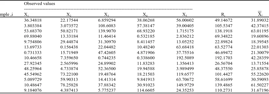
[image:3.612.80.539.564.725.2]

An illustrate example: The data in Table 1 are generated from a gamma distribution with shape parameter, β = 0.98

Table 1: An example of illustration using simulated data from a skewed population (gamma distribution) Observed values

---Sample ,i X1 X2 X3 X4 X5 Ri Xi

1 36.34818 22.17544 6.859294 38.06268 56.00602 49.14672 31.89032

2 3.803384 3.073572 108.6083 57.38147 39.00405 105.5347 42.37415

3 53.68370 50.82171 139.9070 68.93220 1.715175 138.1918 63.01195

4 69.88040 13.33184 11.46414 0.532185 2.836212 69.34822 19.60896

5 9.754806 29.44874 31.30970 8.411457 13.05252 22.89824 18.39545

6 13.69733 0.156438 22.04482 10.48240 63.68418 63.52774 22.01303

7 0.731333 15.71949 47.42605 4.871906 37.75516 46.69472 21.30079

8 10.46658 7.359650 0.744235 0.338600 192.5089 192.1703 42.28359

9 27.92345 2.565996 24.89902 11.83283 1.356413 26.56704 13.71554

10 48.25964 4.733874 52.36500 19.94588 3.989499 48.37550 25.85878

11 45.54962 73.22100 19.48764 18.21503 119.6577 101.4427 55.22620

12 5.089729 59.90313 14.41314 9.841913 63.70672 58.61699 30.59093

13 10.48647 78.25828 37.88342 30.91023 149.9729 139.4865 61.50227

[image:4.612.72.541.97.453.2]

Table 1: Continue

Observed values

---Sample ,i X1 X2 X3 X4 X5 Ri Xi

15 10.29390 23.09588 5.604623 10.95006 51.29480 45.69018 20.24785

16 58.14751 15.92276 42.08211 1.022873 47.96474 57.12463 33.02800

17 77.80144 57.39865 37.56566 37.30812 119.8208 82.51272 65.97894

18 18.38461 60.30539 38.73632 55.00603 50.30109 41.92078 44.54669

19 53.69745 1.597253 33.21739 20.07705 8.381358 52.10020 23.39410

20 28.38292 18.02485 24.47566 15.74064 52.77296 37.03232 27.87941

21 104.7283 6.583657 15.66652 3.788275 8.947521 100.9400 27.94285

22 21.29227 36.70789 74.14813 14.69886 33.40366 59.44927 36.05016

23 11.31113 18.36397 13.27054 49.26539 0.007235 49.25815 18.44365

24 6.521320 7.717710 2.481529 15.99499 66.52404 64.04251 19.84792

25 30.31566 1.008256 3.476084 66.72805 42.92361 65.71980 28.89033

26 24.93475 0.570747 3.297847 18.43215 23.09530 24.36400 14.06616

27 53.42357 80.60140 31.23386 1.746260 15.61345 78.85514 36.52371

28 19.82378 88.34585 9.922032 25.34298 19.09469 78.42382 32.50587

29 12.80654 18.63652 7.658047 7.148106 35.75994 28.61183 16.40183

30 24.91324 2.488491 16.33146 13.29951 3.479776 22.42475 12.10250

= 68.69 = 31.24313

R X

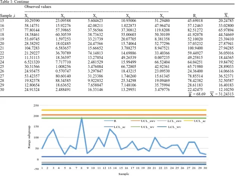
Fig. 1: R type control charts for the SWV, WV and SC methods using simulated data from distribution and scale parameter, λ = 40.50. The data consist of 150

skewed observations grouped into 30 subgroups of size n = 5 each. These data are supposed to correspond to an in-control process. Since, the shape parameter, β is chosen to be 0.98 then the skewness, %₃ = 2. From these data, we compute, ˆx= 25.44, ˆx= 31.24, d₂' = 2.21, d3' = 1.16, d2

* _{= 1.41 and = 68.69. It is observed that}

R

95 observations fall below. Thus, ˆPx= 0.63 using Eq. 5. Consider that α = 0.0027, the SWV-R chart’s control limits computed using Eq. 14 and 15 are equal to UCLSWV-R = 205.456 and LCLSWV-R = -16.127. The control limits of SWV-R chart are compared with those obtained for the WV-R control limits using Eq. 3 and 4, UCLWV-R = 190.103 andLCLWV-R = -24.356 and the SC-R control limits which are computed using Eq. 8 and 9, UCLSC-R = 227.690 and LCLSC-R = 11.363. From Figure 1, we observe that all points fall within control limits of the SWV-R and SC-R control charts indicating that the process is in-control while one points are outside the WV-R chart Upper control limit, potentially signaling a false alarm. To

evaluate the performance of each of these charts, a simulation study is undertaken and the findings are further discussed.

RESULTS AND DISCUSSION

Performance evaluation and discussion of the proposed SWV-R control chart: The SWV!R control chart is compared with the SC-R and WV-R control chart for skewed data. A Monte Carlo simulation is conducted using SAS 9.4 to compute the false alarm rates and Probabilities of out-of-control detections. The false alarm rate of a control chart is defined as the proportion of subgroup points plotting beyond the limits of the chart, given that the process is actually in-control. On the contrary, the probability of out-of-control detection measures the ability of a chart in responding to a shift in the process and it represents the proportion of subgroup points plotting beyond the limits of the chart when the process has shifted. All the charts considered in this study are designed based on an in-control Average Run Length 250

200

150

100

50

0

-50

Rang

e sub

g

roup

Sample

R UCL_swv LCL_swv UCL_sc

LCL_sc UCL_wv LCL_wv

(ARL) of 370 or Type I error of 0.0027. A shift in the process standard deviation is represented by σ₁ = δσ_X where δ0{1.1, 1.2, 1.3, 1.4, 1.5, 2.0, 2.5, 3.0, 3.5, 4.0, 4.5} is the magnitude of a shift in process standard deviation. The skewed distributions considered here are Weibull and gamma because they represent a wide variety of shapes from symmetric to highly skewed. For the sake of comparison, the standard normal distribution is also considered. For convenience, a scale parameter of one is used for the Weibull and gamma distributions. Note that PX for the Weibull and gamma distributions are:

(19)

X

1

P 1-exp - 1+



_{  } 

 

 _ __

 

 

 

and:

(20)

 

X

P F 

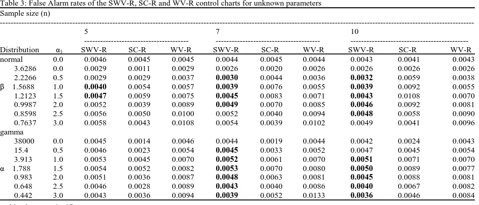
[image:5.612.70.545.315.507.2]

Respectively where β and γ are the shape parameters . Here, Г(.) is the gamma function while F(.) is the gamma distribution functions, respectively. In the case of the false alarm rates, the skewness coefficients considered are α30{0.5, 1.0, 1.5, 2.0, 2.5, 3.0} while skewness coefficient, α₃ = 2 is considered in the case of the probability of out-of-control detection. The sample sizes, n0{5, 7, 10} are considered. The false alarm rate and probability of out-of-control detection are obtained based on 10000 simulation trials. The simulated results are tabulated in Table 2 and 3 for the false alarm rate in the cases of known and unknown parameters while probability of out-of-control detections are tabulated in Table 4-6, respectively where the smallest value are bolded. Table 2 and 3 show that the proposed SWV-R control chart has lower false alarm rate than the SC-R and WV-R control charts for almost all levels of

Table 2: False alarm rates of the SWV-R, SC-R and WV-R control charts for known parameters Sample size (n)

---5 7 10

--- ---- ---

---Distribution α3 SWV-R SC-R WV-R SWV-R SC-R WV-R SWV-R SC-R WV-R

Normal 0.0 0.0064 0.0021 0.0241 0.0059 0.0025 0.0088 0.0055 0.0032 0.0047

Weibull

2.2266 0.5 0.0032 0.0018 0.0033 0.0025 0.0024 0.0032 0.0020 0.0024 0.0024

β 1.5688 1.0 0.0045 0.0045 0.0058 0.0040 0.0057 0.0043 0.0036 0.0048 0.0040

1.2123 1.5 0.0064 0.0099 0.0082 0.0058 0.0134 0.0067 0.0051 0.0085 0.0062

0.9987 2.0 0.0082 0.0166 0.0103 0.0073 0.0246 0.0084 0.0062 0.0118 0.0073

0.8598 2.5 0.0098 0.0222 0.0114 0.0089 0.0372 0.0099 0.0076 0.0143 0.0077

0.7637 3.0 0.0108 0.0250 0.0118 0.0099 0.0436 0.0107 0.0083 0.0167 0.0083

gamma

15.4 0.5 0.0060 0.0056 0.0063 0.0056 0.0041 0.0066 0.0052 0.0048 0.0057

3.913 1.0 0.0066 0.0088 0.0085 0.0060 0.0072 0.0071 0.0057 0.0064 0.0069

α 1.788 1.5 0.0074 0.0097 0.0099 0.0067 0.0126 0.0076 0.0063 0.0086 0.0082

0.983 2.0 0.0084 0.0149 0.0104 0.0072 0.0251 0.0083 0.0064 0.0118 0.0073

0.648 2.5 0.0092 0.0198 0.0096 0.0078 0.0472 0.0096 0.0066 0.0157 0.0057

[image:5.612.72.544.517.719.2]

0.442 3.0 0.0103 0.0225 0.0085 0.0083 0.0802 0.0110 0.0069 0.0208 0.0052

Table 3: False Alarm rates of the SWV-R, SC-R and WV-R control charts for unknown parameters Sample size (n)

---5 7 10

--- ---

---Distribution α3 SWV-R SC-R WV-R SWV-R SC-R WV-R SWV-R SC-R WV-R

normal 0.0 0.0046 0.0045 0.0045 0.0044 0.0045 0.0044 0.0043 0.0041 0.0043

3.6286 0.0 0.0029 0.0011 0.0029 0.0026 0.0020 0.0026 0.0026 0.0026 0.0026

2.2266 0.5 0.0029 0.0029 0.0037 0.0030 0.0044 0.0036 0.0032 0.0059 0.0038

β 1.5688 1.0 0.0040 0.0054 0.0057 0.0039 0.0076 0.0055 0.0039 0.0092 0.0055

1.2123 1.5 0.0047 0.0059 0.0075 0.0045 0.0083 0.0071 0.0043 0.0108 0.0070

0.9987 2.0 0.0052 0.0039 0.0089 0.0049 0.0070 0.0085 0.0046 0.0092 0.0081

0.8598 2.5 0.0056 0.0050 0.0100 0.0052 0.0040 0.0094 0.0048 0.0058 0.0090

0.7637 3.0 0.0058 0.0043 0.0108 0.0054 0.0039 0.0102 0.0049 0.0041 0.0096

gamma

38000 0.0 0.0045 0.0014 0.0046 0.0044 0.0019 0.0044 0.0042 0.0024 0.0043

15.4 0.5 0.0046 0.0023 0.0054 0.0045 0.0033 0.0052 0.0047 0.0045 0.0054

3.913 1.0 0.0053 0.0045 0.0070 0.0052 0.0061 0.0070 0.0051 0.0071 0.0070

α 1.788 1.5 0.0054 0.0052 0.0082 0.0053 0.0070 0.0080 0.0050 0.0089 0.0077

0.983 2.0 0.0051 0.0036 0.0087 0.0048 0.0063 0.0081 0.0045 0.0088 0.0081

0.648 2.5 0.0046 0.0028 0.0089 0.0043 0.0040 0.0086 0.0040 0.0067 0.0082

0.442 3.0 0.0043 0.0036 0.0094 0.0039 0.0052 0.0133 0.0036 0.0046 0.0084

[image:6.612.71.297.117.263.2]

Table 4: Probabilities of out-of-control of variant dispersion control charts, Weibull shape parameter β = 1, n = 5

n = 5

---Distribution/δ SWV-R Exact R-chart SC-R WV-R

Weibull, β = 1 (dalta)

1.1 0.0097 0.0039 0.0061 0.0159

1.2 0.0160 0.0062 0.0095 0.0250

1.3 0.0244 0.0095 0.0143 0.0363

1.4 0.0349 0.0143 0.0212 0.0504

1.5 0.0477 0.0210 0.0303 0.0676

2.0 0.1385 0.0745 0.0977 0.1770

2.5 0.2542 0.1593 0.1962 0.3071

3.0 0.3727 0.2571 0.3025 0.4292

3.5 0.4796 0.3574 0.4078 0.5382

4.0 0.5717 0.4496 0.5008 0.6265

[image:6.612.72.297.291.438.2]

4.5 0.6474 0.5308 0.5802 0.6973

Table 5: Probabilities of out-of-control of variant dispersion control charts, Weibull shape parameter β = 1, n = 7

n = 7

---Distribution/δ SWV-R Exact R-chart SC-R WV-R

Weibull, β = 1 (dalta)

1.1 0.0095 0.0038 0.0080 0.0156

1.2 0.0162 0.0062 0.0109 0.0255

1.3 0.0254 0.0099 0.0160 0.0385

1.4 0.0375 0.0154 0.0234 0.0546

1.5 0.0518 0.0226 0.0329 0.0739

2.0 0.1615 0.0880 0.1149 0.2070

2.5 0.3040 0.1925 0.2354 0.3647

3 0.4473 0.3160 0.3689 0.5121

3.5 0.5716 0.4373 0.4929 0.6333

4.0 0.6722 0.5445 0.5989 0.7262

4.5 0.7504 0.6362 0.6858 0.7964

Table 6: Probabilities of out- of- control of variant dispersion control charts, Weibull shape parameter β = 1, n = 10

n = 10

---Distribution/δ SWV-R Exact R-chart SC-R WV-R

Weibull, β = 1 (dalta)

1.1 0.0094 0.0037 0.0088 0.0155

1.2 0.0165 0.0063 0.0114 0.0262

1.3 0.0269 0.0106 0.0168 0.0407

1.4 0.0404 0.0170 0.0251 0.0596

1.5 0.0572 0.0256 0.0362 0.0817

2.0 0.1883 0.1056 0.1344 0.2412

2.5 0.3622 0.2373 0.2842 0.4315

3 0.5296 0.3886 0.4441 0.6001

3.5 0.5296 0.5333 0.5883 0.7302

4.0 0.6691 0.6525 0.7025 0.8204

4.5 0.7715 0.7471 0.7890 0.8819

skewnesses and sample sizes, when the distributions are Weibull and gamma. Table 4-6 show that the probabilities of out-of-control detections of the proposed SWV-R and SC-R charts are close to those of the exact R chart than the WV-R control chart. In general, the proposed SWV-R control chart provides good performances in term of false alarm rate and probability of out-of-control detection for all levels of skewnesses, sample sizes and magnitudes of shifts.

CONCLUSION

In this study, we have proposed the SWV-R control chart for skewed populations. This proposed chart based on the scaled weighted variance method suggested by Castagliola (2000). The proposed SWV-R control chart reduces to the Shewhart R control chart when the underlying population has a normal distribution. Our simulation study on the false alarm rate indicates that the SWV-R control chart provides lower false alarm rates than those of SC-R and WV-R control charts for all levels of skewnesses and sample sizes. The proposed SWV-R control chart offers considerable improvement over the SC-R and WV-R control charts when it is desirable for the false alarm rate to be closed to the conventional 0.0027. In the case of the probability of out-of-control detections, the simulation results show that the said probabilities of the proposed SWV-R control chart are closer to the chart constructed by exact R chart than the WV-R control charts. The findings are based on the SWV-R method instead of relying on the SC-R and WV-R. Hence, the SWV-R chart can act as a favorable substitute to the existing SC-R and WV-R control charts in the evaluation of the speed of a chart to detect shifts in process dispersion, when the underlying distribution is skewed.

REFERENCES

Atta, A.M.A., M.H.A. Shoraim and S. Yahaya, 2014. A multivariate EWMA control chart for skewed populations using weighted variance method. Int. Res. J. Sci. Eng., 2: 191-202.

Bai, D.S. and I.S. Choi, 1995. X and R control charts for skewed populations. J. Qual. Technol., 27: 120-131.

Castagliola, P., 2000. Control chart for skewed populations using a scaled weighted variance method. Int. J. Reliab. Qual. Saf. Eng., 7: 237-252. Chan, L.K. and H.J. Cui, 2003. Skewness correction X¯

and R charts for skewed distributions. Nav. Res. Logist. (NRL.), 50: 555-573.

Chang, S.Y. and D.S. Bai, 2001. Control charts for positively-skewed populations with weighted standard deviations. Qual. Reliabil. Eng. Int., 17: 397-406.

Chen, Y.K., 2004. Economic design of X¯ control charts for non-normal data using variable sampling policy. Int. J. Prod. Econ., 92: 61-74.

[image:6.612.72.297.468.613.2]

Dou, Y. and P. Sa, 2002. One-sided control charts for the mean of positively skewed distributions. Total Qual. Manage., 13: 1021-1033.

Khoo, M.B.C., A.M.A. Atta and C.H. Chen, 2009. Proposed X and S control charts for skewed distributions. Proceedings of the 2009 IEEE International Conference on Industrial Engineering and Engineering Management, December 8-11, 2009, IEEE, Hong Kong, China, pp: 389-393.

Khoo, M.B.C., A.M.A. Atta and Z. Wu, 2009. A multivariate synthetic control chart for monitoring the process mean vector of skewed populations using weighted standard deviations. Commun. Stat. Simul. Comput., 38: 1493-1518.

Nichols, M.D. and W.J. Padgett, 2006. A bootstrap control chart for Weibull percentiles. Quality Reliabil. Eng. Int., 22: 141-151.

Teh, S.Y., M.B.C. Khoo, K.H. Ong and W.L. Teoh, 2014. Comparing the Median Run Length (MRL) Performances of the Max-EWMA and Max-DEWMA control charts for skewed distributions. Proceedings of the 2014 International Conference on Industrial Engineering and Operations Management, January 7-9, 2014, Bali, Indonesia, pp: 1080-1087.

Tsai, T.R., 2007. Skew normal distribution and the design of control charts for averages. Int. J. Reliab. Qual. Saf. Eng., 14: 49-63.

Wu, Z., 1996. Asymmetric control limits of the x-bar chart for skewed process distributions. Int. J. Qual. Reliab. Manage., 13: 49-60.