warwick.ac.uk/lib-publications
Original citation:
Tremblay, P.-E., Ludwig, H.-G., Freytag, B., Fontaine, G., Steffen, M. and Brassard, P.. (2015)
Calibration of the mixing-length theory for convective white dwarf envelopes. The
Astrophysical Journal, 799 (2). 142.
Permanent WRAP URL:
http://wrap.warwick.ac.uk/83220
Copyright and reuse:
The Warwick Research Archive Portal (WRAP) makes this work by researchers of the
University of Warwick available open access under the following conditions. Copyright ©
and all moral rights to the version of the paper presented here belong to the individual
author(s) and/or other copyright owners. To the extent reasonable and practicable the
material made available in WRAP has been checked for eligibility before being made
available.
Copies of full items can be used for personal research or study, educational, or not-for-profit
purposes without prior permission or charge. Provided that the authors, title and full
bibliographic details are credited, a hyperlink and/or URL is given for the original metadata
page and the content is not changed in any way.
Publisher’s statement:
Reproduced by permission of the AAS.
Published version: http://dx.doi.org/10.1088/0004-637X/799/2/142
A note on versions:
The version presented in WRAP is the published version or, version of record, and may be
cited as it appears here.
C
2015. The American Astronomical Society. All rights reserved.
CALIBRATION OF THE MIXING-LENGTH THEORY FOR CONVECTIVE
WHITE DWARF ENVELOPES
P.-E. Tremblay1,7, H.-G. Ludwig2, B. Freytag3,4, G. Fontaine5, M. Steffen6, and P. Brassard5 1Space Telescope Science Institute, 3700 San Martin Drive, Baltimore, MD 21218, USA;tremblay@stsci.edu 2Zentrum f¨ur Astronomie der Universit¨at Heidelberg, Landessternwarte, K¨onigstuhl 12, D-69117 Heidelberg, Germany 3Department of Physics and Astronomy at Uppsala University, Regementsv¨agen 1, Box 516, SE-75120 Uppsala, Sweden
4Centre de Recherche Astrophysique de Lyon, UMR 5574: CNRS, Universit´e de Lyon,
´
Ecole Normale Sup´erieure de Lyon, 46 all´ee d’Italie, F-69364 Lyon Cedex 07, France
5D´epartement de Physique, Universit´e de Montr´eal, C. P. 6128, Succursale Centre-Ville, Montr´eal, QC H3C 3J7, Canada 6Leibniz-Institut f¨ur Astrophysik Potsdam, An der Sternwarte 16, D-14482 Potsdam, Germany
Received 2014 July 31; accepted 2014 November 25; published 2015 January 23
ABSTRACT
A calibration of the mixing-length parameter in the local mixing-length theory (MLT) is presented for the lower part of the convection zone in pure-hydrogen-atmosphere white dwarfs. The parameterization is performed from a comparison of three-dimensional (3D) CO5BOLD simulations with a grid of one-dimensional (1D) envelopes with a varying mixing-length parameter. In many instances, the 3D simulations are restricted to the upper part of the convection zone. The hydrodynamical calculations suggest, in those cases, that the entropy of the upflows does not change significantly from the bottom of the convection zone to regions immediately below the photosphere. We rely on this asymptotic entropy value, characteristic of the deep and adiabatically stratified layers, to calibrate 1D envelopes. The calibration encompasses the convective hydrogen-line (DA) white dwarfs in the effective temperature range 6000 Teff (K) 15,000 and the surface gravity range 7.0 logg 9.0. It is established
that the local MLT is unable to reproduce simultaneously the thermodynamical, flux, and dynamical properties of the 3D simulations. We therefore propose three different parameterizations for these quantities. The resulting calibration can be applied to structure and envelope calculations, in particular for pulsation, chemical diffusion, and convective mixing studies. On the other hand, convection has no effect on the white dwarf cooling rates until there is a convective coupling with the degenerate core belowTeff ∼5000 K. In this regime, the 1D structures are
insensitive to the MLT parameterization and converge to the mean 3D results, hence they remain fully appropriate for age determinations.
Key words: convection – hydrodynamics – stars: evolution – stars: fundamental parameters –
stars: interiors – white dwarfs
1. INTRODUCTION
In late-type stars, giants, and cool white dwarfs, the con-vective outer envelope has a significant impact on the observed properties. The physical principles explaining convective energy transport in stars are well understood, although the nonlocal and turbulent nature of convection has delayed the development of precise models for convective stellar layers. The mixing-length theory (B¨ohm-Vitense1958, hereafter MLT) has proven rather successful despite presenting a very simple description of con-vection. In this picture, the condition that distinguishes between convective and stable layers is the Schwarzschild criterion, and the convective efficiency, the ratio of convective and radiative fluxes, is computed from local quantities. In the superadiabatic convective layers that define the atmosphere of most stars, the predicted convective efficiency is very sensitive to the underly-ing model describunderly-ing the radiative energy losses, the lifetime, and the geometrical shape of individual convective structures. These quantities are not well constrained by theMLTand must be calibrated from observations.
In recent years, three-dimensional (3D) radiation hydrody-namical (RHD) simulations have provided predictions for the surface convection that are in very good agreement with the ob-served solar granulation (see, e.g., Wedemeyer-B¨ohm & Rouppe van der Voort 2009). Furthermore, various studies relied on 3D RHD simulations to improve the predicted photospheric
7 Hubble Fellow.
structures and spectroscopic abundance determinations for the Sun and other stars (Asplund et al.2009; Caffau et al.2011; Scott et al.2015a,2015b). In addition to a better representation of the surface inhomogeneities, 3D model atmospheres feature nonlo-cal effects, such as the so-nonlo-called top overshoot layers, which are completely missing in local one-dimensional (1D)MLTmodels (Unno1957; Ludwig et al.2002; Nordlund et al.2009; Freytag et al.2010; Tremblay et al.2013c).
The deep convection zone, where the stratification becomes essentially adiabatic, is not sensitive to the convection model. It is, however, the entropy jump in the superadiabatic layers that completely defines the asymptotic entropy value of the deep, adiabatically stratified structure, hence also the depth of the convection zone. One possibility to model these layers is to rely on RHD simulations to determine the asymptotic entropy value for the deep convection zone (Steffen1993; Ludwig et al.
1999). This arises from the prediction that upflows formed at the base of the convection zone follow an adiabat almost up to the visible surface (Stein & Nordlund1989). The 1DMLT
a pure-hydrogen atmosphere. All currently available white dwarf structures rely on the local MLT with a fixed parame-terization (see, e.g., Tassoul et al.1990; Fontaine et al.2001; Renedo et al.2010; Salaris et al.2010).
Surface granulation in DA white dwarfs is qualitatively very similar to that seen in the Sun and stars (Tremblay et al.2013a), albeit with shorter lifetimes and smaller characteristic sizes, which are roughly inversely proportional to gravity. Convec-tive instabilities due to hydrogen recombination develop in the atmosphere of these pure-hydrogen stellar remnants atTeff ∼
18,000 K, although convective energy fluxes only become sig-nificant atTeff ∼14,000 K for logg=8. The convection zone
eventually grows to subphotospheric and essentially adiabatic layers, at slightly lower effective temperatures. White dwarfs in the range 14,000 Teff (K) 8000 have superadiabatic
photospheric layers where the 1DMLTparameterization has a strong influence on the predicted thermal structures and spectra (Bergeron et al.1992,1995; Koester et al.1994). Tremblay et al. (2013c) recently demonstrated that the local 1DMLTis unable to reproduce the mean photospheric structure of 3D simula-tions, and that shortcomings in the 1DMLTare responsible for the spurious high loggvalues previously derived from spectro-scopic observations of cool convective white dwarfs (Bergeron et al.1990). In particular, the top overshoot region was found to have a crucial impact on the spectroscopic predictions.
The convection zone in DA white dwarfs remains limited to the thin hydrogen envelope until it reaches the degenerate core at Teff ∼5000 K, or mixes with the underlying helium layer if the
total gravitationally stratified mass of hydrogen is less than about 10−6MH/Mtot(Tassoul et al.1990). Before one of these events
takes place, the cooling process is regulated by the radiative interface layer just above the largely isothermal degenerate core, which is in some sense the bottleneck for the energy transport. The evolutionary calculations converge to the so-called radiative zero solution; hence, they are insensitive to the details of the convection model (Fontaine & van Horn1976), which is unlike earlier evolutionary stages (see, e.g., Freytag & Salaris1999). The situation is different below Teff ∼ 5000 K, where the
cooling rates are directly impacted by the convecting coupling between the interior thermal reservoir and the radiating surface. In this temperature range, however, the superadiabatic peak has a negligible amplitude, or in other words, the full convection zone has an essentially adiabatic structure that does not depend on theMLTparameterization. As a consequence, the cooling ages predicted from current 1D evolutionary sequences are not expected to be impacted by 3D effects. However, the convection zone has anindirect effect on observed ages, since they are often derived from spectroscopically determined atmospheric parameters that are modified by 3D effects.
There are a number of cases where 3D effects on structures are expected to have a direct impact. Nonadiabatic pulsation calculations depend critically on the structure of the convective layers, especially for the determination of the edges of the ZZ Ceti instability strip of pulsating DA white dwarfs (Fontaine et al. 1994; Gautschy et al. 1996; van Grootel et al. 2012). Chemical diffusion applications (Paquette et al.1986; Pelletier et al.1986; Dupuis et al.1993) and convective mixing studies (see, e.g., Chen & Hansen2011) also depend critically on the size and especially the dynamical properties of the convection zone, e.g., the rms vertical velocity in the convective overshoot layers at the base of the convection zone (Freytag et al.1996). In order to characterize white dwarfs accreting disrupted planets, it is likely important to account for the currently neglected
convective overshoot (Koester 2009). The total mass of the chemical elements mixed in the convection zone (hereafter mixed mass), and to a lesser degree their relative abundances, depend on how rapidly these elements diffuse in the deep overshoot region. Throughout the remaining of this work, overshoot refers only to the region at the base of the convection zone, since the top overshoot layers have no direct relevance for white dwarf envelope and structure models.
This study proposes a calibration of theMLTfree parameters for the size of the convection zone in 1D envelopes of DA white dwarfs from a comparison with CO5BOLD 3D simulations
previously computed for spectroscopic applications (Tremblay et al. 2013c). We emphasize that our proposed calibration has little in common with the spectroscopic parameterization of the MLT. In both cases, the free parameters of the MLT
are employed to mimic specific properties of the mean 3D simulations and mean 3D spectra, respectively, rather than to describe the more general underlying nature of convection. In Section 2 we introduce our grid of 3D simulations and 1D envelope models. We follow in Section3 with definitions for the sizes of nonlocal convection zones. In Section4we compare 1D and 3D models, in order to propose and discuss an MLT
parameterization in Section5. We conclude in Section6.
2. WHITE DWARF MODELS
2.1. 3D Model Atmosphere Simulations
We rely on CO5BOLD 3D simulations that were presented in earlier works (Tremblay et al.2013a,2013b,2013c, hereafter TL13a, TL13b, and TL13c, respectively). The 70 simulations cover the range 6000Teff(K)15,000 and 7logg9 (see
Appendix A ofTL13c). WhileTL13creviewed the predicted spectral properties drawn from these simulations, which mostly depend on the uppermost regions of the convection zone, the study presented here reports on the overall properties and lower parts of convection zones. The natural starting point is therefore the comparison of 3D and 1D structures at logg=8 presented in TL13b. We have demonstrated that sequences at different surface gravities possess rather similar properties (TL13a,TL13c), largely because 3D effects depend mostly on the local density, and the same range of densities is found at all surface gravities, albeit with a shift inTeff.
The numerical setup of the 3D model atmospheres is de-scribed in detail inTL13band more broadly in Freytag et al. (2012) in terms of the general properties of the code. We pro-vide a brief overview in this section. The 3D simulations rely on an equation of state (EOS) and opacity tables that are com-puted with the same microphysics as that of standard 1D model atmospheres (Tremblay et al. 2011). We employed a grid of 150×150×150 points in thex, y,andzdirections, wherez is used for the vertical direction and points toward the exterior of the star. The grid spacing in thezdirection is nonequidistant, and the total horizontal extent is chosen in order to have about 10 granules at the surface. The structure of the deep convec-tion zone is largely determined by the radiative energy losses in the photosphere, which also fix theTeff of a simulation. As
Figure 1.Entropy at the bottom of the convection zone as a function ofTefffor
DA white dwarf envelopes at logg=8. The 3D results are shown in black, with the3Dentropy extracted directly at the Schwarzschild boundary for closed simulations (open circles; see Section4.1), and asymptoticsenvvalues for open
simulations (filled squares; see Section4.2). We also display 1D sequences (solid lines; see Section2.3) with theMLTparameterization varying from ML2/α= 0.4 (red) to 2.0 (blue) in steps of 0.2 dex. Additionally, we present sequences where gas degeneracy effects are neglected (dotted lines), which largely follow the former sequences.
applications (TL13c). This setup is likely more than sufficient for a comparison with 1D structure calculations, which are less sensitive to the optically thin layers.
The implementation of boundary conditions is described in detail in Freytag et al. (2012, see Section 3.2). In brief, the lateral boundaries are periodic, and the top boundary is open to material flows and radiation. We rely on bottom conditions that are either open or closed to convective flows. The lower boundary is closed (hereafter closed simulations) when the vertical extent of the convection zone can be fully included in the simulation. This is the situation for the 3D simulations withTeff 10,500,11,500,12,000,13,000, and 14,000 K, for logg =7.0, 7.5, 8.0, 8.5, and 9.0, respectively. In those cases, we impose zero vertical velocities at the bottom, and a radiative flux is injected from below.
For cooler simulations, the bottom layer is open to convective flows and radiation (hereafter open simulations), and a zero total mass flux is enforced. We specify the entropy of the ascending material to obtain approximately the desiredTeffvalue
(an indirect quantity computed from the resulting emergent flux of the simulation). Figure1shows that the entropy from 1D envelopes (see Section 2.3) at the lower boundary of the convection zone increases monotonically withTeff. Convection
is essentially adiabatic in deep convection zones, and the entropy value in the lower part of the convection zone is assumed to be the same as that of the upflows at the bottom of the simulations (see Section2.2).
In all models, the top boundary reaches a space- and time-averaged value of no more than a Rosseland optical depth of τR ∼10−5. The bottom layer was generally fixed atτR=103,
well below the photosphere, i.e., the line-forming regions. A few models were extended to deeper layers when the bottom of the convection zone was too close to the simulation boundary. We cover at least ∼3 pressure scale heights (HP) below the
unstable regions when the bottom of the simulation is closed to mass flows.
Figure 2.Local 3D entropy values (black dots) as a function of geometrical depth for a subset of a simulation atTeff=10,025 K and logg=8. The3Dentropy
profile, averaged over constant geometrical depth, is shown with a red solid line. We also display the 1D entropy (dashed red line) with theMLTparameterization calibrated from the 3D simulation (ML2/α=0.69; see Table2). We highlight τRvalues at 100, 1.0, and 0.1 (cyan points, values identified in the legend) as a
guide. The asymptotic 3D entropy valuesenvis 2.082×10⁹erg g−1K−1.
2.2. Properties of the Deep Convection Zone
The physical conditions at the bottom of convection zones can be extracted from 3D simulations even if we do not simulate the full zones. We rely on the technique presented in Ludwig et al. (1999), for which a demonstration is shown in Figure2
for a DA simulation at Teff = 10,025 K and logg = 8.
We present the local 3D values of the entropy in convective structures (black dots) as a function of geometrical depth with the stellar surface on the right-hand side. We also display the average entropy profile over constant geometrical depth (solid red line). We observe significant entropy fluctuations at all depths, although there is a constant asymptotic upper limit, hereafter senv. According to the scenario developed in Stein
& Nordlund (1989) and Ludwig et al. (1999), the gas in central regions of broad ascending flows is still thermally isolated from its surroundings until it reaches layers immediately below the photosphere. In other words, convective upflows keep an imprint of the physical conditions at the bottom of the convection zone. The averaged 3D entropy, on the other hand, is not a conserved quantity owing to radiative losses and the presence of downdrafts created in the photosphere.
The above technique only applies if the center of upflows remains adiabatic; hence, a minimum requirement is that the conditions at the bottom of the convection zone are adiabatic. We have observed that the adiabatic transition takes place when the bottom of the convection zone reaches layers deeper than τR∼103. For all of our simulations with an open bottom, we can
recover an asymptotic value. For closed simulations, there is no significant entropy plateau since conditions are never adiabatic, although in those cases we can directly extract the properties at the bottom of the convection zones.
We also overlay in Figure2the 1D model atmosphere with the MLT calibrated from a comparison ofsenv with a grid of
[image:4.612.45.294.53.245.2]On the other hand, there is no guarantee that the calibrated 1D models will provide a good match to the mean 3D stratification in superadiabatic layers. Fortunately, in the case of white dwarfs, in contrast to main-sequence stars, the superadiabatic layers have little direct impact on applications that require the use of 1D envelopes. As was customary until now, it is generally sufficient to employ 1D envelopes where the MLT parameterization is based on the deep layers and rely on a different set of models, e.g., 3D simulations, for atmospheric parameter determinations. An inspection of Figure 2 demonstrates that, if needed, a connection of the 1D and mean 3D structures at large depth could also be a fairly good approximation.
2.3. 1D Envelope Models
For the purpose of this work, we computed 1D envelopes relying on the MLT for the treatment of convection, similar to those presented in Fontaine et al. (2001) and van Grootel et al. (2012). The models employ the ML2 treatment ofMLT
convection (B¨ohm & Cassinelli 1971; Tassoul et al. 1990) and an EOS for a nonideal pure-hydrogen gas (Saumon et al.
1995). Realistic nongray temperature gradients are extracted from detailed atmospheric computations and employed as upper boundary conditions (Brassard & Fontaine1997; van Grootel et al.2012). The nongray effects on the size of the convection zone are shown in Figure 5 of van Grootel et al. (2012). In order to compare the envelopes to 3D simulations, we have varied the ratio of mixing length to pressure scale height,8ML2/α=l/H
P,
from values of 0.4 to 2.0 in steps of 0.2. ML2/αis selected as a proxy for allMLTfree parameters since changes in the other parameters have similar effects on the structures. We use the same range of surface gravities andTeff (steps of 0.5 dex and
100 K, respectively) as our set of 3D calculations.
From the 1D envelopes we have extracted the physical conditions at the bottom of the convection zone. Figure 3
depicts the hydrogen mass integrated from the surface (MH),
with respect to the total white dwarf mass, for the logg = 8 case. Clearly, theMLTparameterization has a strong effect on the size and mass included in the convection zone at intermediate temperatures, where the atmospheric layers are superadiabatic. To ensure that we share a common entropy zero point in all calculations, we computed all entropy values using the same EOS as the 3D simulations, based on the Hummer & Mihalas (1988) nonideal EOS, where we have also accounted for partial degeneracy. The entropy values at the bottom of the convection zone are shown in Figure1(solid lines), along with additional sequences where we have neglected partial degeneracy (dotted lines). The degeneracy effects are very small in the convection zone (η <0, whereηkT is the chemical potential of the free electrons). This is largely due to the fact that the degeneracy level is constant for an adiabatic process. For theessentiallyadiabatic structure of cool white dwarf convection zones, degeneracy is changing very slowly as a function of depth (see Equation (13) of B¨ohm1968). Furthermore, degeneracy effects are still negligible at the lower Teff limit where the calibration of ML2/α is
performed in this work (see Section5.1).
Our proposed calibration of theMLTis performed by com-paring 3D simulations to 1D envelopes. We also rely on 1D
MLTmodel atmospheres (Tremblay et al.2011) for illustrative purposes in cases where we display a detailed comparison of
8 ML2/αhas the same functional form as the more commonly usedα MLTfor
stars, but it also specifies the choice of auxiliary parameters of theMLT
[image:5.612.321.568.53.242.2]formulation (Ludwig et al.1999).
Figure 3.Mass of hydrogen integrated from the surface (MH) with respect to
the total stellar mass (logarithmic value) as a function ofTefffor DA envelopes
at logg = 8. The 3D results are shown with black symbols using different definitions for the bottom of the convection zone (see Sections3and4). For closed simulations, we consider the Schwarzschild boundary (open circles), the flux boundary (filled circles), and avz,rmsdecay of 1 dex (open triangles) below
the value at the flux boundary. For open 3D simulations, the filled squares represent the values calibrated by matchingsenvwith the 1D entropy at the
bottom of the convection zone. We also display 1D sequences (solid lines) with theMLTparameterization varying from ML2/α=0.4 (red) to 2.0 (blue) in steps of 0.2 dex. The bottom of the stellar photosphere (τR=1, 1D ML2/α=
0.8), which roughly coincides with the top of the convection zone, is represented by a dotted black line.
1D and mean 3D stratifications as a function of depth. The 1D model atmospheres and envelopes provide very similar results, within a few percent, below the photosphere.
3. DEFINITION OF CONVECTIVE LAYERS
In the following, we rely on mean 3D values, hereafter3D, for all quantities except for the asymptotic entropysenv.3D
values are the temporal and spatial average of 3D simulations over constant geometrical depth. We use 250 snapshots in the last 25% of a simulation to make the temporal average. While our earlier studies have relied on averages over constant optical depth, the geometrical depth is better suited to extract convective fluxes and overshoot velocities.
Before comparing 3D simulations and 1D envelopes, it is crucial to define what we refer to as the convection zone. In the local MLT picture, the convective regions are clearly characterized as the layers where the radiative gradient,
∇rad=
∂lnT ∂lnP
rad
, (1)
is larger than the adiabatic gradient,
∇ad=
∂lnT ∂lnP
ad
, (2)
Table 1
Regions in the Lower Part of Convection Zones
Region ds
dz
a ds
dz
a F
conv/Ftotal Fconv/Ftotal vz vz Δzb ΔlogMH/Mtotb
(3D) (1D) (3D) (1D) (3D) (1D)
Zone 1 <0 <0 >0 >0 =0 =0 . . . . . .
Zone 2 >0 >0 >0 0 =0 0 0.8HP 0.2
Zone 3 >0 >0 <0 0 =0 0 ∼1.6HP ∼0.5
Zone 4 >0 >0 ∼0 0 =0 0 >3HP >1.0
Notes.
aThe coordinatezpoints toward the exterior of the star.
bRanges are taken from the simulation atT
eff=12,100 K and logg∼8.0 as an illustrative example. Zones 3 and 4 feature
[image:6.612.47.295.219.481.2]an exponential decay of (negative) flux and velocity, respectively, and their depth can only be defined approximately. For the example presented here, we adopt a bottom boundary of|Fconv/Ftotal|<0.01 for Zone 3.
Figure 4.Vertical rms velocity as a function of the logarithm of the temperature for 3D simulations at logg=8 (solid red lines). TheTeffvalues are identified
on the top right of the panels. We show the position of the Schwarzschild boundary (open circles), the flux boundary (filled circles), and thevz,rmsdecay
of 1 dex (open triangles) below the value at the flux boundary. We also display 1D model atmospheres with the calibration of theMLTparameters (see Table2) for the Schwarzschild (dotted black) and flux boundaries (dashed blue). For the models warmer than 13,000 K, we rely on an asymptotic parameterization of ML2/αSchwa=1.2 and ML2/αflux=1.4, respectively (see Section5.1).
Table1 formally defines the regions discussed in this section, and we give an example of the geometrical extent and mass included in these layers based on the 12,100 K and logg =8 simulation.
To further illustrate the profile of 3D convection zones, Figure 4 displays the rms vertical velocities for closed-box simulations at logg = 8. We start from the vertical velocity
vz=uz−
ρuz
ρ , (3)
where the mass flux weighted mean velocity (second term on right-hand side) is removed from the directly simulated velocity uzto account for the residual numerical mass flux. The latter
[image:6.612.320.569.221.460.2]results from the presence of plane-parallel oscillations and an imperfect temporal averaging due to the finite number of
Figure 5.Ratio of the convective energy flux to total flux as a function of the logarithm of the temperature at logg=8. The3Dfluxes are represented by solid red lines, andTeffvalues for the simulations are identified on the panel.
The ratio is exact for the 12,100 K model, but other structures are shifted by one flux unit for clarity. The symbols are the same as in Figure4. We also display 1D model atmospheres matching the Schwarzschild boundary (black, dotted) and the flux boundary (blue, dashed). Parameters for the Schwarzschild boundary are ML2/αSchwa=0.88, 1.07, and 1.32 for the 12,100, 12,500, and 13,000 K
models, respectively. The values are ML2/αflux=1.00, 1.25, and 1.50 for the
flux boundary at the same temperatures.
snapshots. The corresponding rms vertical velocity is
vz2,rms= vz2 = u2z+ρuz
2
ρ2 −2
ρuzuz
ρ , (4)
where all averages are performed over constant geometrical depth.9 Furthermore, Figures5 and6 show the 3D and 1D convective flux profiles. The3Dconvective flux is the sum of the enthalpy and kinetic energy fluxes,
Fconv=
eint+
P
ρ
ρuz
+
u2
2 ρuz
−etotρuz, (5)
9 This differs from the rms velocity fluctuationv2
z − vz2, wherevzis
Figure 6.Similar to Figure5, but for the 3D simulations (solid red) at 13,500 and 14,000 K. The convective-to-total flux ratio is exact for the model at 13,500 K and shifted by 0.1 flux units for the 14,000 K case. The symbols are the same as in Figure4. In this regime, theMLTis unable to replicate both the 3D size of the convection zone and the maximumFconv/Ftotratio. We display instead 1D
ML2/α=0.7 model atmospheres (black, dot-dashed), which correspond to the averageMLTparameterization to reproduce the maximumFconv/Ftotratio for
shallow convection zones (see Section4.1).
where eint is the internal energy per gram,ρ the density, and
uthe 3D velocity. The mass flux weighted energy flux (third term on right-hand side of Equation (5)) is subtracted to correct for any residual nonzero mass flux in the numerical simulations as in Equation (4). This correction is a small fraction of the convective flux for all simulations. The total energy is defined from
etot=
ρeint+P +ρu
2
2
ρ . (6)
We use the logarithm of the temperature as an independent variable since it is a local quantity, while optical depth and mass are integrated from the top of the convection zone and are more sensitive to differences in the photosphere.
The proper convection zone in 3D (open circles in Figures 4–6) is defined in the same way as in 1D from the Schwarzschild (stability) criterion. In this region, the entropy gradient is negative with respect to geometrical depth (increas-ing toward the exterior). In the follow(increas-ing, we define the bottom of this region as theSchwarzschild boundary. In the 3D sim-ulations, convective flows are largely created, horizontally ad-vected, and merged into narrow downdrafts in the photosphere (Freytag et al.1996). Large entropy fluctuations are produced by the radiative cooling in these layers, which drives the convective motions. For cool convective white dwarfs (Teff 11,000 K,
logg=8) with deep convection zones, entropy fluctuations are smaller in the photosphere and the dominant role of the down-flows is diminished. The descending fluid forms a hierarchical structure of merging downdrafts owing to the increase of the pressure scale height with depth (Nordlund et al.2009).
In the 3D simulations, downdrafts at the base of the con-vection zone (according to the Schwarzschild criterion) still have large momenta. They are also denser than the ambient medium, albeit with a decreasing difference. As a consequence,
the convective cells are still accelerated in the region just below the unstable layers. Mass conservation guarantees that there is warm material transported upward; hence, there is a positive convective flux in this region. These layers are equivalent to a convection zone in thermodynamical terms. We define the bot-tom of this region as the layer whereFconv/Ftot =0 and refer
to it as the flux boundary (filled circles in Figures 4–6). The typical size of the region between the Schwarzschild and flux boundaries is a bit less than one pressure scale height, or∼0.3 dex in mass.
At the flux boundary, the momentum of the downdrafts remains significant; hence, they penetrate into even deeper layers. This is the beginning of the convective overshoot region, although some authors prefer the term “convective penetration” (Zahn 1991) when the convective flux is still energetically relevant. In these layers, convective structures are decelerated since they have a density deficit. Downdrafts are generally warmer than the ambient medium and carry a net downward (negative) convective flux; in other words, the temperature gradient in these layers is larger than the radiative gradient. That follows from the change of sign of the velocity–enthalpy correlation. However, Figure5demonstrates that this negative overshoot flux is always a small fraction (10%) of the total flux. Once the convective flux has decreased by one order of magnitude, or to a value of less than 1% of the total flux, the energetic impact on the structure becomes very small.
The negative convective flux and velocities decay in a similar exponential way below the flux boundary, both with a scale height close toHP. While the convective flux becomes rapidly
energetically negligible, the convective velocities still have mixing capabilities in much deeper layers. This situation is due to the extreme ratio between convective and diffusive timescales (see Section 5.2). In typical cases for DA white dwarfs, convective velocities are of the order of vz,rms ∼
1 km s−1 at the base of the convection zone, while overshoot velocities of the order of 1 m s−1still dominate over the slower
diffusive speeds and can efficiently mix elements (Freytag et al.
1996). This implies that microscopic diffusion timescales are likely to dominate only in the deep overshoot layers, i.e., a few HP below the flux boundary. The exact layer where this
happens depends on the diffusing trace chemical element and the atmospheric parameters of the model, although it is clear that the mixed region can be much larger than in the 1D approximation. In Figures 4–6, we identify the position of a 1 dex velocity decay with respect to the velocity at the flux boundary (filled triangles), which is generally close to the bottom of the simulation. Our simulations evidently provide a truncated picture of the overshoot layers, and we review this issue in Section5.2.
4. COMPARISON OF 1D AND 3D CONVECTION ZONES
4.1. Closed 3D Simulations
We first proceed with a direct comparison of 3D and 1D stratifications in the case of shallow convection zones, completely enclosed within the simulation domain. Figures7
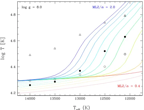
Figure 7.Logarithm value of the temperature at the bottom of the convection zone as a function ofTeff, for DA white dwarf envelopes at logg =8. The
3Dresults are shown with black symbols using different definitions for the bottom of the convection zone (see Section3). We consider the Schwarzschild boundary (open circles), the flux boundary (filled circles), and avz,rmsdecay
of 1 dex (open triangles) below the value at the flux boundary. We also display 1D sequences with theMLTparameterization varying from ML2/α=0.4 (red) to 2.0 (blue) in steps of 0.2 dex. The solid lines represent the bottom of the convection zone defined by the Schwarzschild boundary, while the dotted lines stand for the layers below which the convective flux becomes energetically negligible (Fconv/Ftot<0.01).
of 1 dex (open triangles) below the reference value at the flux boundary. Figures 7 and 8 also display 1D sequences, with values ranging from ML2/α=0.4 to 2.0 in steps of 0.2, using the Schwarzschild boundary to define the size of the convection zone (solid lines).
Figures7 and8demonstrate that the 1D envelope that best matches the bottom of a 3D simulation is generally indepen-dent of whether the matching is performed on temperature or pressure. The pressure is proportional to the 1D mass column, where only thermodynamic pressure contributes to hydrostatic equilibrium, while in 3D simulations one must also account for the turbulent pressure. Figure3depicts the3Dand 1D com-parison in terms of the hydrogen mass, and the results are similar to those presented for the temperature and pressure at the base of the convection zone. It implies that even though3D and 1D models have different profiles in the photosphere, owing to the top convective overshoot and turbulent pressure, differences in the integrated mass column are small in the lower part of the convection zone. In the following, the calibrated ML2/α is the average value of the two 1D models that best match the
3Dpressure and temperature at the bottom of the convection zone, respectively, within a prescribed boundary. The mass col-umn can be directly extracted from the envelopes calibrated in this way.
In terms of the Schwarzschild boundary, Figures 7 and 8
demonstrate that the mixing-length parameter increases rapidly withTeff, with values of 0.88, 1.07, and 1.32 at 12,100, 12,500,
and 13,000 K, respectively. In thisTeff range partially covering
[image:8.612.320.568.54.244.2]the ZZ Ceti instability strip, the MLT variation is significant compared to the usually assumed constant value of ML2/α= 1.0 for envelopes (Fontaine & Brassard2008). Our calibration of ML2/αis meant to represent the3Dtemperature and pres-sure at the Schwarzschild boundary, and by construction, it pro-vides an estimation of the average temperature gradient for the full convection zone. However, the photospheric temperature
Figure 8.Similar to Figure7, but for the thermal pressure (logarithm value) at the bottom of the convection zone as a function ofTeffat logg=8.
gradient of a calibrated 1D envelope is not expected to corre-spond to that of the 3D simulation.
For the convection zone defined in terms of the3D flux boundary, ML2/αvalues have to be increased to 1.00, 1.25, and 1.50 for the sameTeff values as above. The derived efficiency
is significantly higher than that found for the Schwarzschild boundary. One should be cautious since an inspection of Figure5
for 1D model atmospheres calibrated for the flux boundary (blue dashed lines) reveals that while the zero point of convective flux is by definition in agreement with the 3D simulations, the overall shape of the3Dconvective flux is not very well reproduced for shallow convection zones. Our calibration of ML2/α is mostly useful to characterize the depth at which convection becomes energetically insignificant and the velocities start to decay exponentially with geometrical depth. Finally, Figure9
demonstrates that the3Dversus 1D results (temperature only) at other gravities are fairly similar, albeit with a shift inTeff. As
a consequence, the previous discussion applies most generally to white dwarfs with shallow convection zones.
For the very warm simulations, e.g., 13,500 and 14,000 K at logg = 8.0, the Schwarzschild and flux boundaries are essentially in the photosphere (τR,bottom<10), and therefore the
ML2/αvalue for these layers becomes coupled with theMLT
parameterization used in spectroscopic applications (TL13c). Both 3D simulations and 1D models show new patterns in thisTeff regime. The3Dconvective flux becomes negligible
outside of the unstable layers, and there is a reversal of the flux and Schwarzschild boundaries, with the Schwarzschild boundary moving below the flux boundary with increasingTeff.
Figure 9.Similar to Figure7, but for logg=7.0, 7.5, 8.5, and 9.0, with values identified in the panels.
neglected. TheMLT does not account for the kinetic energy flux; hence, we do not expect a similar reversal in 1D.
For convective 1D models at largeTeff, the size of the
un-stable regions becomes insensitive to theMLT parameteriza-tion according to Figure7; hence, it is not possible to calibrate theMLTbased on the Schwarzschild boundary. This picture is somewhat misleading since theMLTconvective fluxes and as-sociated velocities remain very sensitive to the value of theMLT
parameters. Figure7shows that the 1D convective flux drops to very small values (Fconv/Ftot<0.01; dotted lines) much higher
in the photosphere than the 1D Schwarzschild boundary. Our results would naively suggest that convective efficiency increases with Teff, but the 3D simulations present a more
complex picture. At high Teff, nonlocal effects from strong
and deep-reaching downdrafts create 3D flux profiles that are extended and smoother as a function of geometrical depth than in the 1D case, at both the top and bottom of the convection zone. In Figure 10 we have calibrated ML2/α in order to reproduce the maximum value of the3Dconvective flux, which peaks in the photosphere, for shallow convection zones. Clearly, a much smaller mixing-length parameter is necessary to match the3Dconvective flux in the photosphere in comparison to the Schwarzschild or flux boundaries. The values of ML2/α=0.6–0.8 are consistent with the commonly used spectroscopic parameterizations (TL13c). Nevertheless, the parameterizations for the Schwarzschild and flux boundaries offer a better representation of the conditions at the bottom of the convection zones.
We have already discussed the fact that the convection zone is drastically deeper when defined in terms of the3D convective velocities. This is also seen in Figures 7 and 8, where we show the position of the one order of magnitude decrease forvz,rms below the flux boundary (open triangles).
It is inappropriate to parameterize the 1DMLTfor the highly
Figure 10.Calibration of ML2/αfor the maximumFconv/Ftotratio as a function
ofTeffand logg(represented by different colors with the legend at the bottom).
The calibration is based on the 1D model that best replicates the maximum3D convective flux of closed simulations. This calibration cannot be performed for deep convection zones since all 1D models haveFconv,max/Ftot∼1.
nonlocal overshoot velocities, and it would produce spurious stratifications in the unstable regions. Instead, we propose an overshoot parameterization that does not directly involve the
MLTin Section5.2.
4.2. Open 3D Simulations
For open 3D simulations, we have extracted the asymptotic entropy valuessenvcharacterizing the deep adiabatic layers using
the technique described in Section2.2.senvis directly derived
from the specified entropy of the ascending material at the bottom boundary of the simulations. We have verified that this matches the observed asymptotic value below the photosphere (see, e.g., Figure2). We then assume thatsenvalso corresponds
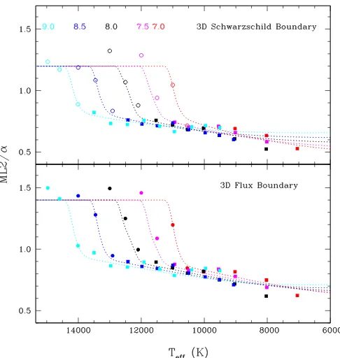
[image:9.612.320.568.375.523.2]Figure 11.Top: calibration of ML2/αSchwafor the lower part of the convection
zone as a function ofTeffand logg(represented by different colors with the
legend at the top). The calibration is based on the 1D model that best replicates the Schwarzschild boundary of a 3D simulation, either from a direct comparison (open circles) or by using thesenvcalibration (filled squares). The dotted lines
correspond to the proposed fitting function (Equation (9)). Bottom: calibration of ML2/αfluxbased on the 1D model that best represents the flux boundary of
a 3D simulation (filled circles). For open 3D simulations, we use ML2/αflux=
1.16 ML2/αSchwa. The dotted lines correspond to the proposed fitting function
(Equation (10)).
1D envelopes. The senv and 1D entropy values are compared
in Figure1for the logg =8 case. The calibration of ML2/α is directly performed from a match ofsenvwith entropy values
interpolated from the grid of 1D envelopes. In Figure3we show the resulting hydrogen mass integrated from the surface.
At low temperatures (Teff 7000 K at logg=8), DA white
dwarfs have extremely small superadiabatic atmospheric layers, and the structure remains essentially adiabatic from the bottom to the top of the convection zone. Since the top of the convection zone is higher than the photosphere (τR ∼ 0.1), the effective temperature directly identifies the entropy value at the bottom of the convection zone. The choice of theMLTparameterization does not matter since there is no significant radiative energy exchange during one advective (turnover) timescale.
5. DISCUSSION
5.1. 1D MLT Calibration
Figure11(top panel) presents theMLTparameterization for the lower part of the convection zone in order to recover the Schwarzschild boundary (hereafter ML2/αSchwa) of the 70 3D
simulations in our grid. We illustrate with different symbols the calibration derived directly from closed 3D simulations (open circles) and inferred from a match ofsenv (filled squares). We
also present in Figure11(bottom panel) the calibration match-ing the 3D flux boundary (hereafter ML2/αflux). The latter
calibration is directly performed for closed simulations, and in those cases, αflux is 16% larger than αSchwa, with a
rela-tively small dispersion of 3%. Therefore, we simply assume that ML2/αflux = 1.16ML2/αSchwa for open 3D simulations. This
is likely a good approximation in the transition region between closed and open 3D simulations, and at lowerTeff, the 1D
en-velopes depend less critically on theMLTparameterization. The calibration is not performed when the 1D mass included within the convection zone varies by an amount smaller than 0.2 dex for the range of ML2/αbetween 0.4 and 2.0. This defines the upper and lowerTeffboundaries in Figure11, which depend
on logg. At the cool end, we propose to keep ML2/αconstant, since the value is irrelevant for structure calculations. Similarly, atTeff values above those in the calibration range, it is likely
acceptable to keep the value constant for most applications. The choice of the asymptotic ML2/αvalue is not obvious, however, because of its rapid variation withTeff. As a compromise, we
adopt values of 1.2 and 1.4, for ML2/αSchwa and ML2/αflux,
respectively, atTeff values larger than our calibration range. If
one is interested in the detailed properties of shallow convection zones aboveTeff ∼12,000 K at logg=8.0, it may be preferable
to combine the3Dand 1D structures at some depth below the convection zone where the convective flux is negligible. The
MLTdoes not reproduce very well the extended but inefficient 3D convection zones in this regime. ForTeff values above our
calibration range, most of the 3D effects will be from the overshoot at the base of the convection zone since, contrary to the small convective fluxes, velocities remain significant well below the photosphere.
Table2provides the tabulatedMLTparameterizations, which are valid for 1D envelopes with an EOS, opacities, and boundary conditions similar to those employed for our grid. Physical conditions at the bottom of our calibrated envelopes (mass, temperature, and pressure) are also given as a reference point. Moreover, we propose fitting functions for ML2/αSchwa and
ML2/αflux, respectively, where the independent variables are defined as
g0=logg(cgs)−8.0, (7)
T0=(Teff(K)−12,000)/1000−1.6g0, (8)
and the functions are as follows, with numerical coefficients found in Table3:
ML2/αSchwa=(a1+ (a2+a3exp[a4T0+a5g0])
×exp[(a6+a7exp[a8T0])T0+a9g0]) +a10
×exp(−a11([T0−a12]2+ [g0−a13]2)), (9)
ML2/αflux=(a1+a2exp[(a3+{a4+a5exp[a6T0+a7g0]}
×exp[a8T0])T0+a9g0]) +a10
×exp(−a11([T0−a12]2+ [g0−a13]2)). (10)
Table 2
ML2/αCalibration for DA Envelopes
Teff logg ML2/αSchwaa logMH/Mtota logTa logPa ML2/αfluxb logMH/Mtotb logTb logPb
(K) (K) (dyn cm−2) (K) (dyn cm−2)
6112 7.00 0.53 −6.06 5.93 14.04 0.61 −6.03 5.94 14.07
7046 7.00 0.53 −6.79 5.80 13.30 0.61 −6.74 5.81 13.36
8027 7.00 0.63 −7.51 5.68 12.58 0.74 −7.42 5.69 12.67
9025 7.00 0.69 −8.90 5.41 11.19 0.80 −8.69 5.45 11.40
9521 7.00 0.70 −10.14 5.17 9.94 0.81 −9.78 5.24 10.31
10018 7.00 0.69 −12.00 4.84 8.07 0.80 −11.49 4.93 8.59
10540 7.00 0.72 −13.92 4.44 6.16 0.85 −13.33 4.58 6.74
11000 7.00 1.05 −14.30 4.34 5.78 1.20 −13.98 4.42 6.10
11501 7.00 1.20 −14.63 4.28 5.45 1.40 −14.59 4.29 5.49
12001 7.00 1.20 −14.78 4.26 5.30 1.40 −14.77 4.26 5.30
12501 7.00 1.20 −14.89 4.24 5.19 1.40 −14.89 4.24 5.19
13003 7.00 1.20 −14.98 4.23 5.10 1.40 −14.98 4.23 5.10
6065 7.50 0.58 −6.91 5.90 14.17 0.67 −6.90 5.90 14.19
7033 7.50 0.58 −7.54 5.79 13.54 0.67 −7.51 5.80 13.57
8017 7.50 0.58 −8.22 5.68 12.86 0.68 −8.16 5.69 12.92
9015 7.50 0.66 −9.07 5.53 12.01 0.77 −8.95 5.55 12.13
9549 7.50 0.71 −9.83 5.38 11.25 0.82 −9.64 5.42 11.44
10007 7.50 0.70 −10.81 5.19 10.27 0.81 −10.52 5.25 10.55
10500 7.50 0.70 −12.30 4.93 8.78 0.82 −11.86 5.00 9.21
10938 7.50 0.74 −13.68 4.68 7.40 0.86 −13.12 4.79 7.96
11498 7.50 0.94 −14.79 4.42 6.29 1.09 −14.27 4.56 6.81
11999 7.50 1.20 −15.24 4.32 5.84 1.40 −15.06 4.36 6.02
12500 7.50 1.20 −15.43 4.29 5.65 1.40 −15.42 4.29 5.66
13002 7.50 1.20 −15.53 4.28 5.55 1.40 −15.52 4.28 5.55
5997 8.00 0.52 −7.68 5.89 14.40 0.60 −7.67 5.89 14.41
7011 8.00 0.52 −8.44 5.75 13.64 0.60 −8.42 5.76 13.65
8034 8.00 0.52 −9.01 5.66 13.07 0.60 −8.97 5.67 13.11
9036 8.00 0.61 −9.66 5.55 12.41 0.71 −9.58 5.57 12.50
9518 8.00 0.64 −10.10 5.47 11.98 0.74 −9.98 5.50 12.10
10025 8.00 0.69 −10.71 5.36 11.36 0.80 −10.56 5.39 11.52
10532 8.00 0.68 −11.61 5.19 10.46 0.79 −11.39 5.23 10.68
11005 8.00 0.72 −12.63 5.00 9.45 0.84 −12.32 5.06 9.75
11529 8.00 0.76 −14.04 4.76 8.04 0.88 −13.58 4.84 8.50
12099 8.00 0.88 −15.27 4.51 6.81 1.00 −14.82 4.63 7.26
12504 8.00 1.07 −15.69 4.40 6.38 1.25 −15.27 4.52 6.81
13000 8.00 1.20 −16.05 4.33 6.03 1.40 −15.96 4.35 6.12
13502 8.00 1.20 −16.18 4.31 5.89 1.40 −16.17 4.31 5.90
14000 8.00 1.20 −16.26 4.30 5.81 1.40 −16.26 4.30 5.82
6024 8.50 0.60 −8.51 5.86 14.57 0.70 −8.51 5.86 14.57
6925 8.50 0.60 −9.32 5.71 13.76 0.70 −9.31 5.72 13.76
8004 8.50 0.60 −9.80 5.65 13.28 0.70 −9.78 5.65 13.30
9068 8.50 0.60 −10.38 5.55 12.69 0.70 −10.33 5.56 12.74
9522 8.50 0.64 −10.67 5.51 12.41 0.74 −10.61 5.52 12.47
9972 8.50 0.66 −11.01 5.45 12.07 0.76 −10.93 5.46 12.14
10496 8.50 0.68 −11.52 5.35 11.55 0.79 −11.41 5.38 11.67
10997 8.50 0.74 −12.19 5.23 10.89 0.86 −12.04 5.26 11.04
11490 8.50 0.72 −13.04 5.08 10.04 0.84 −12.81 5.12 10.26
11979 8.50 0.73 −14.09 4.89 8.99 0.84 −13.78 4.95 9.29
12420 8.50 0.76 −15.11 4.72 7.96 0.88 −14.68 4.79 8.40
12909 8.50 0.84 −16.11 4.50 6.96 0.95 −15.71 4.61 7.37
13453 8.50 1.08 −16.47 4.42 6.61 1.28 −16.10 4.51 6.97
14002 8.50 1.19 −16.76 4.36 6.31 1.40 −16.67 4.38 6.41
14492 8.50 1.20 −16.89 4.33 6.18 1.40 −16.87 4.34 6.20
6028 9.00 0.70 −9.38 5.80 14.70 0.81 −9.38 5.80 14.70
6960 9.00 0.70 −10.24 5.67 13.84 0.81 −10.23 5.67 13.84
8041 9.00 0.70 −10.75 5.59 13.33 0.81 −10.74 5.60 13.34
8999 9.00 0.70 −11.10 5.55 12.98 0.81 −11.09 5.55 12.99
9507 9.00 0.71 −11.34 5.51 12.74 0.82 −11.31 5.52 12.77
9962 9.00 0.72 −11.59 5.47 12.48 0.84 −11.56 5.48 12.52
10403 9.00 0.71 −11.89 5.42 12.18 0.82 −11.85 5.43 12.23
10948 9.00 0.67 −12.37 5.34 11.70 0.77 −12.30 5.35 11.78
11415 9.00 0.71 −12.84 5.25 11.23 0.83 −12.73 5.27 11.35
11915 9.00 0.76 −13.47 5.14 10.61 0.88 −13.33 5.16 10.75
Table 2
(Continued)
Teff logg ML2/αSchwaa logMH/Mtota logTa logPa ML2/αfluxb logMH/Mtotb logTb logPb
(K) (K) (dyn cm−2) (K) (dyn cm−2)
12969 9.00 0.73 −15.29 4.83 8.79 0.85 −15.02 4.87 9.06
13496 9.00 0.82 −16.05 4.70 8.03 0.96 −15.75 4.75 8.32
14008 9.00 0.89 −16.92 4.51 7.15 1.03 −16.52 4.62 7.56
14591 9.00 1.17 −17.23 4.44 6.85 1.40 −16.87 4.53 7.20
14967 9.00 1.20 −17.47 4.38 6.61 1.40 −17.34 4.41 6.73
Notes.Teffis the spatial and temporal average of the emergent flux. The rmsTeffvariations are found in Table 1 ofTL13a. logMH/Mtot,
logT, and logPare extracted at the bottom of the convection zone from calibrated 1D envelopes.
aCorresponds to the position of the3DSchwarzschild boundary for closed simulations (see Section4.1). For open simulations, the
calibration is performed by matching the 3Dsenvvalue with the 1D entropy at the bottom of the convection zone (see Section4.2). b Corresponds to the position of the 3D flux boundary for closed simulations. For open simulations, we simply assume that
[image:12.612.322.568.241.430.2]ML2/αflux=1.16 ML2/αSchwa(see Section5.1).
Table 3
Coefficients for Fitting Functions
Coefficient ML2/αSchwa ML2/αflux
a1 1.1989083E+00 1.4000539E+00
a2 −1.8659403E+00 −5.1134694E−01
a3 1.4425660E+00 −1.1159288E+00
a4 6.4742170E−02 1.0083984E+00
a5 −2.9996192E−02 −5.7427026E−02
a6 6.0750771E−02 5.4884977E+00
a7 −5.2572772E−02 −1.6106825E−02
a8 5.4690218E+00 −7.5656008E−03
a9 −1.6330177E−01 −6.8772823E−02
a10 2.8348941E−01 2.9166886E−01
a11 1.7353691E+01 1.8977236E+01
a12 4.3545950E−01 3.6544167E−01
a13 −2.1739157E−01 −2.2859657E−01
5.2. Parameterization of Overshoot Velocities
We have so far neglected the convective overshoot below the flux boundary. In most cases, the quantity of interest is the overshoot velocity, which does not exist in the localMLT. In the following, we aim at providing a parameterization for overshoot in regions below the 1D convection zone.
The spatial scales and timescales involved in convection and microscopic diffusion differ by many orders of magnitude in typical white dwarfs. It is therefore not possible for multidi-mensional simulations to model both effects simultaneously. Instead, we depict the far overshoot regime as a random walk process characterized by a macroscopic diffusion coefficient, which simply counterbalances the microscopic diffusion coef-ficient in 1D calculations. The mixed regions are those where macroscopic diffusion dominates over microscopic diffusion. Freytag et al. (1996) studied this random walk process with tracer particles in 2D RHD simulations. They found that the particles are immediately mixed within the convection zone, but that the rms vertical spreadδzovershoot in the overshoot layers
could be described from
δz2overshoot=2Dovershoot(z)t, (11)
whereDovershootis the macroscopic diffusion coefficient
Dovershoot(z)=v2z,rms(z)tchar(z), (12)
withtchara characteristic timescale. Just based onMLTmodels
or even with detailed RHD simulations,vz,rms is not directly
Figure 12. Vertical rms velocity decay as a function of pressure (natural logarithm values) for 3D simulations at logg=8. The reference point is the flux boundary for which we defineΔlnvz,rms=0 andΔlnP=0. The simulations
are color-coded fromTeff=12,100 (red), 12,500, 13,000, 13,500, to 14,000 K
(blue). The−1 dotted black slope represents an exponential velocity decay with a scale height ofHP. The velocity decay atΔlnP >2 could be impacted by the
closed bottom boundary condition.
available for the deep overshoot regions of interest. As a consequence, Freytag et al. (1996) propose, from a match to 2D simulations and physical considerations, thatvz,rms has an
exponential decay below the convection zone. The resulting diffusion coefficient then takes the form
Dovershoot(z)=v2basetcharexp(2(z−zbase)/Hv), (13)
where vbaseis the velocity at the base of the convection zone
andHvis the velocity scale height. In the following, we assume
that the base of the convection zone is the flux boundary as determined by 3D simulations and the 1D ML2/αflux
parame-terization.
5.2.1. Closed 3D Simulations
For closed 3D simulations, it is possible to verify the proposed exponential decay of overshoot velocities, as well as calibrate Equation (13) by extracting vbase, tchar, and Hv. Figure 12
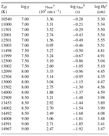
[image:12.612.71.265.260.411.2]Table 4
Overshoot Parameters for Closed 3D Simulations
Teff logg vbasea logtcharb logHPc
(K) (105cm s−1) (s) (cm)
10540 7.00 3.36 −0.28 5.30
11000 7.00 3.31 −0.21 5.34
11501 7.00 3.52 −0.29 5.50
12001 7.00 2.74 −0.43 5.54
12501 7.00 1.56 −0.49 5.55
13003 7.00 0.95 −0.46 5.51
11498 7.50 3.27 −0.50 4.81
11999 7.50 3.24 −0.67 4.91
12500 7.50 3.10 −0.86 5.04
13002 7.50 2.60 −1.05 5.10
12099 8.00 3.33 −0.96 4.45
12504 8.00 3.14 −0.95 4.35
13000 8.00 3.04 −1.15 4.47
13502 8.00 2.75 −1.30 4.56
14000 8.00 1.88 −1.37 4.59
12909 8.50 3.21 −1.48 3.98
13453 8.50 2.92 −1.44 3.89
14002 8.50 2.70 −1.54 3.99
14492 8.50 2.49 −1.68 4.08
14008 9.00 3.06 −1.81 3.48
14591 9.00 2.71 −1.85 3.41
14967 9.00 2.47 −1.92 3.47
Notes.
aCorresponds to3Dv
z,rmsat the flux boundary. bSame as the decay time in Table A.1 ofTL13c. cCorresponds to3DP /(ρg) at the flux boundary.
close to one pressure scale height (dotted black line), although it is actually changing with depth. It is larger than one pressure scale height immediately below the flux boundary and becomes subsequently smaller. As a consequence, takingHv = HP is very likely to overestimate macroscopic diffusion in the deep overshoot layers and gives an upper limit to the mixed mass. Finally, Freytag et al. (1996) demonstrate that the timescale of overshoot for shallow convection zones is the same as the characteristic convective timescale in the photosphere, since this is where the downdrafts are formed. As a consequence, it is possible to use directly the characteristic granulation timescales computed inTL13a andTL13c. In Table 4 we presentvz,rms
at the flux boundary (vbase) and the characteristic granulation timescales (tchar) for closed simulations, which can be used in
Equation (13) for shallow convection zones. The velocity scale height can be directly evaluated from the 1D pressure scale height in the envelopes since this quantity is not significantly impacted by 3D effects, although we also include the local3D values at the base of the convection zone in Table4.
The overshoot coefficients in Table4are limited by theTeff
range of our 3D simulations. Figure13compares the maximum velocities, which peak slightly below the photosphere, for3D and 1D ML2/α =0.7 models at logg = 8. We applied the
MLTparameterization that best represents the maximum con-vective flux of the warmest 3D simulations (see Figure10and
TL13c). TheMLTsuggests that velocities in the photosphere for 14,000< Teff (K)18,000 are still of the same order of mag-nitude as in cooler models, although the upperTefflimit depends
[image:13.612.65.273.71.330.2]critically on theMLTparameterization. The large photospheric velocities are likely to support strong overshoot layers in DA white dwarfs above our warmest 3D simulations, even though convection has a negligible effect on the thermal structure.
Figure 13. Maximum vz,rms velocity within the convection zone for 3D
simulations (filled points, red) and 1D ML2/α=0.7 model atmospheres (open points, black) at logg=8. The points are connected for clarity.
5.2.2. Open 3D Simulations
For open 3D simulations, we cannot directly extract quan-tities to calibrate Equation (13). Furthermore, the assumption that the overshoot timescale is the same as the surface gran-ulation timescale is unlikely to be valid, since the downdrafts have time for merging into the hierarchical structure observed in simulations of deep, convective envelopes (Nordlund et al.
2009). We propose instead thattchar = Hv/vbase, with the ve-locity scale height equal to the pressure scale height as above. Therefore,vbaseis the only quantity that remains to be evaluated.
For deep and essentially adiabatic convection zones, theMLT
and 3D simulations agree on the temperature gradient. An examination of theMLT equations demonstrates that for very efficient convection (Fconv ∼ Ftot), velocity is proportional to
ρ−1/3, along with a dependence on heat capacity and molecular
weight in the presence of partial ionization. While the 1D velocity model is only an idealization of the complex 3D dynamics, we suggest that thev3D/v1Dratio remains very similar
across the deep convection zone. This is seen in Figure 4for the cooler 10,025 K model, where convection is reasonably adiabatic below the photosphere. Figure 14 shows the 3D versus 1D ML2/αflux velocity ratio for open simulations and a reference layer identified by the criterion logτR =2.5. This
region is deep enough for convection to be largely adiabatic and far away from the bottom boundary to prevent numerical effects. We observe small variations around a mean value ofv3D/v1D=
1.5 for the DA white dwarfs with a deep adiabatic convection zone. We suggest that this calibration remains valid down to the bottom of the convection zone, as long asFconv∼Ftot. We still
face the problem, however, that by definitionvMLT,base=0. We
recommend instead to take a characteristic velocity vMLT,base∗
one pressure scale height above the bottom of the convection zone. In summary, for theTeff range below the one covered by
Table4, we propose the following overshoot parameterization:
Dovershoot(z)=1.5vMLT,base∗HPexp(2(z−zbase)/HP), (14)
where all quantities are extracted from 1D ML2/αfluxstructures as described above.
Figure 14.Ratio of the 3Dvz,rmsand 1D ML2/αfluxvelocities at logτR=2.5
as a function ofTeffand logg(represented by different colors with the legend
at the top). The points are connected for clarity. The ML2/αfluxcalibration is
presented in Table2.
convectively unstable layers (Teff 18,000 K). The total mass
of hydrogen included in the overshoot region may be a few or-ders of magnitude greater than the mass included in the proper convection zone. This effect is totally neglected in localMLT
models, and our proposed parameterization provides an order-of-magnitude estimate (upper limit) of the overshoot velocities and macroscopic diffusion coefficients. The resulting effects on the chemical abundances of mixed elements, for instance, in ac-creting white dwarfs in a steady state, depend on the outcomes of chemical diffusion calculations.
5.3. Improvements to the Local MLT
The previous sections have revealed that the localMLTonly depicts a rough portrait of the underlying dynamical nature of convection, which is illustrated by the need of having different parameterizations for different applications. We note that nonlocal 1DMLTmodels could provide a better match to the 3D results. In particular, the models discussed in Spiegel (1963), Skaley & Stix (1991), Dupret et al. (2006), and St¨okl (2008) naturally deliver the Schwarzschild and flux boundaries, as well as (partial) overshoot layers. In these nonlocalMLT models, the more realistic physics is recovered at the expense of adding more free parameters. In some sense, this is a more elegant and accurate way of obtaining the Schwarzschild and flux boundaries than we have proposed in this work. While it does require some modifications of existing 1D model atmosphere and structure codes, this should be investigated in the future.
Montgomery & Kupka (2004) have also presented a nonlo-cal convection model for white dwarfs, although in this case it is not an extension of theMLTtheory. However, one issue for all nonlocal 1D models discussed here is that they have not been very successful at modeling overshoot velocities re-producing the exponential decay observed in RHD simulations, which is the main part of the 1D models that we would like to improve.
5.4. ZZ Ceti Instability Strip
The spectroscopically determined atmospheric parameters of pulsating ZZ Ceti white dwarfs have been discussed inTL13c,
as seen in the light of our grid of3Dspectra. We found that the dominant 3D effect is on the spectroscopically determined surface gravity, with an average shift ofΔlogg= −0.1 for ZZ Ceti stars in the sample of Gianninas et al. (2011). On the other hand, 3DTeffcorrections depend critically on the calibration of
the MLTparameters in the reference 1D model atmospheres. Based on the 1D ML2/α = 0.8 calibration, we observed a 3D shift of ΔTeff = −225 K on average, although this is in
the same range as the uncertainties in the 3D corrections. The
spectroscopicblue edge at logg=8, below which white dwarfs
are pulsating, is located at Teff ∼ 12,500 K when relying on
3Dspectra, while it is slightly warmer by 100 K based on 1D ML2/α=0.8 model atmospheres. On the other hand, the3D red edge is located atTeff ∼11,000 K for logg =8. Overall,
the observed position of the instability strip is not changed significantly compared to earlier investigations (Gianninas et al.
2006, 2011). We remind the reader that the observed edges are defined from only a few pulsating and constant objects, and that the individual errors on the spectroscopic atmospheric parameters must also be considered.
Nonadiabatic asteroseismic models provide predictions for the position of the blue edge of the ZZ Ceti instability strip, although the results are highly sensitive to the parameterization of convection (Fontaine et al.1994; Gautschy et al.1996). Re-cently, van Grootel et al. (2012) relied on a nonadiabatic code including time-dependent convection to study the driving mech-anism. Compared to earlier studies (Fontaine & Brassard2008
and references therein), their approach assumes neither frozen convection nor an instantaneous convection response during a pulsation cycle. Using 1D ML2/α = 1.0 white dwarf struc-tures similar to those discussed in this work, they find aseismic
blue edge at Teff = 11,970 K for logg = 8. Since the con-vective flux contribution is critical in the nonadiabatic pertur-bation equations, we can compare their results with our ML2/ αflux calibration in Figure11. We find that ML2/αflux∼1.0 at
12,000 K and logg = 8, in very close agreement with the value generally used to predict the blue edge of the instabil-ity strip, based on seismic models. There seems to be a slight discrepancy between the observed and predicted blue edges, the latter being cooler by about 500 K. We note, however, that the current agreement is still fairly good considering the uncer-tainties in the 3D simulations and spectroscopically determined atmospheric parameters. It would be interesting to review the nonadiabatic pulsation calculations with the new calibrated 1D envelopes or a direct use of the3D convective flux profiles (Gautschy et al. 1996). Finally, dynamical convection effects that are missing from both current and newly calibrated 1D en-velopes could also have an impact on pulsations (van Grootel et al.2012).
At the red edge of the instability strip, van Grootel et al. (2013) recently revived an idea of Hansen et al. (1985) originally applied to the blue edge. They suggest that the red edge of the
g-mode instabilities is reached when the thermal timescale in the driving region (bottom of the convection zone) becomes of the order of the pulsation period. Beyond this limit, outgoing
g-waves are no longer reflected back by the atmospheric layers and will lose their energy in the upper atmosphere. Using this argument forg-modes of spherical-harmonic degree
l = 1, the red edge lies at ∼11,000 K for logg = 8 with ML2/α=1.0 1D envelopes. In this range ofTeff, we predict a