Novel approach for health monitoring of earthen embankments

http://wrap.warwick.ac.uk/

Utili, Stefano, Castellanza, R., Galli, A. and Sentenac, P.. (2015) Novel approach for health monitoring of earthen embankments. Journal of Geotechnical and

Geoenvironmental Engineering , 141 (3). 04014111.

http://dx.doi.org/10.1061/(ASCE)GT.1943-5606.0001215

Permanent WRAP url:

http://wrap.warwick.ac.uk/71254

Copyright and reuse:

The Warwick Research Archive Portal (WRAP) makes this work of researchers of the University of Warwick available open access under the following conditions. Copyright © and all moral rights to the version of the paper presented here belong to the individual author(s) and/or other copyright owners. To the extent reasonable and practicable the material made available in WRAP has been checked for eligibility before being made available.

Copies of full items can be used for personal research or study, educational, or not-for-profit purposes without prior permission or charge. Provided that the authors, title and full bibliographic details are credited, a hyperlink and/or URL is given for the original metadata page and the content is not changed in any way.

Publisher statement:

A note on versions:

The version presented here may differ from the published version or, version of record, if you wish to cite this item you are advised to consult the publisher’s version. Please see the ‘permanent WRAP url’ above for details on accessing the published version and note that access may require a subscription.

Novel approach for health monitoring of earthen embankments

1 2 3

Utili S. 1_{, Castellanza R.} 2_{, Galli A.} 3_{, Sentenac P.} 4_,

4

5

1 School of Engineering

6

University of Warwick, UK

7

formerly at University of Oxford, UK

8 9 10

2 Department of Geology and Geotechnologies

11

Università Milano-Bicocca, Italy

12 13 14

3 Department of Structural Engineering

15

Politecnico di Milano, Italy

16 17 18

4 Department of Civil Engineering

19

University of Strathclyde, UK

20 21 22

ABSTRACT. This paper introduces a novel modular approach for the monitoring of 23

desiccation-induced deterioration in earthen embankments (levees), which are typically 24

employed as flood defence structures. The approach is based on the use of a combination of 25

geotechnical and non-invasive geophysical probes for the continuous monitoring of the water 26

content in the ground. The level of accuracy of the monitoring is adaptable to the available 27

financial resources. 28

The proposed methodology was used and validated on a recently built 2 km long river 29

embankment in Galston (Scotland, UK). A suite of geotechnical probes was installed to 30

monitor the seasonal variation of water content over a two-year period. Most devices were 31

calibrated in-situ. A novel procedure to extrapolate the value of water content from the 32

geotechnical and geophysical probes in any point of the embankment is illustrated. 33

Desiccation fissuring degrades the resistance of embankments against several failure 34

mechanisms. An index of susceptibility is here proposed. The index is a useful tool to assess 35

the health state of the structure and prioritise remedial interventions. 36

2

KEYWORDS: embankments; earthfills; resilient infrastructures; geophysics; slope stability; desiccation fissuring.

3

1.

Introduction

42

Earthen flood defence embankments also known as levees are long structures usually made of 43

local material available at the construction site. In the UK, flood defence embankments are 44

mainly made of cohesive soils: either clay or silt. Most of them were built before the 45

development of modern soil mechanics in the eighteenth century (Charles, 2008). Due to 46

their progressive aging, proper infrastructure condition assessment, based on sound 47

engineering, is becoming increasingly important (Perry et al., 2001). 48

The formation of desiccation cracks in earthen embankments and tailing dams 49

(Rodriguez et al., 2007) made of cohesive soils during dry seasons is detrimental to their 50

stability. Desiccation is responsible for the onset of primary cracks which first appear at the 51

surface, and then propagate downwards, and for so-called secondary and tertiary cracks 52

(Konrad and Ayad, 1997). Desiccation induced failures are deemed to become increasingly

53

important as progressively more extreme weather conditions are predicted by climatologists 54

to take place worldwide (Milly et al, 2002). Allsop et al. (2007) provide a comprehensive list 55

of the several failure modes that may take place in earthen embankments. Several potential 56

failure mechanisms are negatively affected by the presence of desiccation cracks such as: 57

deep rotational slides starting from the horizontal upper surface (Utili, 2013); shallow slides 58

developing along the flanks (Aubeny and Lytton 2004; Zhang et al., 2005); erosion of the 59

flanks by overtopping water (Wu et al., 2011) and/or wave action (D’Elisio, 2007); and 60

internal erosion (Wan and Fell, 2004). In particular, the presence of cracks can substantially 61

decrease the resistance of embankments with regard to overtopping and internal erosion 62

which alone count for 34 and 28 percent respectively of all the embankment failures in the 63

world (Wu et al., 2011). 64

Monitoring and condition assessment of flood defence embankments worldwide are 65

4

1999). In a few countries (e.g. the UK (Environment Agency, 2006), the Netherlands, the US) 67

guidelines exist to rate the health/deterioration of embankments on the basis of a prescribed 68

set of visual features. Unfortunately, this type of assessment is purely qualitative and relies 69

heavily on the level of training and experience of the inspection engineer. So, there is 70

consensus among experts on the fact that although visual inspection provides valuable 71

information, a meaningful and robust assessment of the fitness for purpose of earthen flood 72

defence embankments cannot rely entirely on visual inspection (Allsop et al., 2007). On the 73

other hand, intrusive tests (e.g. Cone Penetration test, piezocones, vane tests, inclinometers) 74

are impractical for the monitoring of long structures like embankments given the necessity of 75

performing tests in several locations to account for the typical high variability of the ground 76

properties. The same applies to standard geotechnical laboratory tests which involve time-77

consuming retrieval and transportation of samples to the laboratory. 78

In this paper, a cost effective approach employing a suite of geotechnical and geophysical 79

probes is proposed for the long term monitoring of the variation of water content in the 80

ground and of the liability to desiccation induced fissuring. The methodology is simple, 81

modular (i.e. the level of sophistication/accuracy is a function of the financial resources

82

available), and it can be readily implemented by the authorities in charge of the management 83

of earthen flood defence embankments and tailing dams. 84

85

2.

Conceptual framework

86

The methodology here proposed is based on the assumption that water content can be 87

selected as a direct indicator of the occurrence of extensive fissuring in the ground as 88

suggested by Dyer et al., (2009) and Tang et al., (2012). The authors are aware that a lot of 89

research has been recently performed to successfully relate the onset of cracks to soil suction 90

5

well illustrated by Costa et al., (2013), the formation and propagation of cracks in cohesive 92

soils depends on several other factors too, such as the drying rate and the amount of fracture 93

energy involved in the crack propagation. Considering flood defence embankments, loss of 94

structural integrity (i.e. loss of the structure capacity to withstand the design hydraulic load)

95

occurs when desiccation fissuring progresses to the extent that an interconnected network of 96

cracks is formed rather than when surficial cracks first appear. Therefore the approximation 97

introduced in relating the loss of structural integrity to a threshold value of suction appears no 98

less important than the approximation introduced in relating it to a threshold value in terms of 99

water content. Moreover, the cost of monitoring suction in a long embankment for an 100

extended period of time is very significant with the extra burden of necessitating complex 101

installation and maintenance procedures for the probes needed to measure suction. These 102

reasons underpin the authors’ choice of monitoring the ground water content. 103

The position of any point in a long linear structure like an embankment or tailing dam 104

can be defined according to either a global Cartesian coordinate system (X,Y,Z) or a local 105

coordinate system defined at the level of the structure cross-sections. For sake of simplicity, 106

the following choice was made: a curvilinear global coordinate, s, running along the

107

longitudinal direction of the structure which uniquely identifies the location of any cross 108

section; a local Cartesian coordinate, x, lying in the horizontal plane and perpendicular to the

109

s coordinate; and a vertical downward Cartesian coordinate, z, which can be thought of as

110

both a global and local coordinate. So, the water content, w, in a generic point of the earthen

111

structure is a function of these three spatial coordinates and of time: w(x,s,z,t). A local

112

tangential coordinate st was also defined as shown in Figure 1b. The procedure proposed to 113

determine the function w=w(x,s,z,t) in the whole embankment is based on the following

114

6

1) measurement of the water content profile along a vertical line P of coordinate xP, sP at

116

any time and depth w x x s s z t

(

)

( )

117

2) measurements in some selected cross-sections, located at s s= _i (herein the subscript i

118

is an integer identifying the embankment cross-section considered), at some discrete 119

time points t_k (herein the subscript k is an integer identifying the time point

120

considered), of the function w x s s z t t

(

)

( )

121

3) measurement by geophysical techniques of the water content at predefined time

122

points, t_k, along the entire embankment (i.e. for any value of s);

123

4) evaluation by extrapolation of the water content in any point at any time: w x s z t

(

)

124

Once the water content function w x s z t

(

)

125

susceptibility of any cross-section of the embankment to desiccation fissuring can be defined 126

and a map of susceptibility can be generated to identify the most critical zones of the 127

structure (see section 8). The map is useful to set priorities for intervention in the zones 128

requiring remedial actions. 129

130

3.

Description of the site

131

In 2007, the construction of an earthen flood defence embankment enclosing a floodplain 132

along the river Irvine to drain excess waters from the river during floods was completed in 133

Galston (Scotland, UK). The embankment is made of an uppermost layer (5-10 cm) of a 134

sandy topsoil below which lies a core of glacial till containing several boulders (Figure 1). 135

Grass roots do not extend beyond the topsoil. A typical cross- section is sketched in Figure 136

1b. Although the inclination of the flanks is rather uniform, the size of the flanks and of the 137

7

negligible spatial variation of the geometry of the cross-sections which may have 139

consequences in terms of the spatial variation of the water content in the ground (see sections 140

6 and 7). 141

142

a)

143

144

b)

145

Figure 1. a) Plan view of the monitored embankment; b) typical embankment cross section and system of

146

coordinates adopted in the paper.

147 148

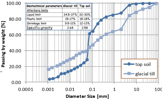
A number of standard geotechnical tests were carried out to characterise the ground 149

properties: measurements of gravimetric moisture content, void ratio, particle size 150

distribution and Atterberg limits were taken. The grain size distribution of both the top soil 151

and the glacial till was determined according to ASTM E11 (see Figure 2). 152

200m  

Section  B  

 Section  A  

N  

 Legend  

   CMD  electromagnetic    Resistivity  arrays    Coordinates  

Section  A:  Lat.    55°  36’  20.0’’  N                                        Long.  4°  25’  32.5’’  W   Section  B:  Lat.    55°  36’  15.4’’  N                                        Long.  4°  25’  44.7’’  W    

r     st  

θ

8 153

Figure 2. Particle size distribution of the glacial till and of the topsoil and main geotechnical indices.

154 155

4.

Monitoring system

156

In the following, the main geotechnical and geophysical measurements of the monitoring 157

system are described. The main technical features of all the probes employed in the 158

monitoring programme (e.g. manufacturer, accuracy, operational range, etc.) are listed in 159

Table 1. 160

161

4.1 Measurement of the water content along the selected vertical P 162

In Figure 3b, the vertical line P is plotted with the label PR2_E2. A data-logger, reading data 163

at an hourly frequency was installed into a bespoke metallic fence close to the vertical line P 164

(see Figure 3c). As schematically shown in Figure 3a and b, the following devices were 165

connected to the data-logger: 166

a) a theta probe (THP) made of four metal rods to be inserted in the ground to measure

167

its water content at a depth of 25 cm. Special care was taken to avoid the formation of 168

any air gaps between the prongs of the probe and the surrounding soil by prefilling the 169

augered holes hosting the probes with a slurry and pushing the probe into undisturbed 170

soil well beyond the hole bottom. The device takes a measurement of the relative 171

0.00 20.00 40.00 60.00 80.00 100.00

0.0001 0.001 0.01 0.1 1 10 100

Pe

rc

ent

 P

as

si

ng

 i

n  

w

ei

ght

 [%

]

Diameter  Size  [mm]

top  soil glacial  till Specific gravity

Passi

ng

 b

y  we

ig

ht  [

%

9

permittivity (also commonly called dielectric constant) of the ground which is then 172

converted into gravimetric water content; 173

b) an equitensiometer (EQ) to measure suction up to a maximum value of 1000 kPa at

174

the same depth of 25 cm. This device consists of theta probe pins embedded into a 175

porous matric; 176

c) a portable profile probe (PR), which is based on time domain reflectometry, to

177

measure the water content at six different depths from the ground surface (10, 20, 30, 178

40, 60 and 100 cm); 179

d) two temperature probes inserted at 25 and 40 cm of depth in the ground.

180

181

4.2 Measurement of the water content at cross-section A and B 182

To evaluate the water content in the ground up to 1 meter of depth, several access tubes were 183

drilled into two cross-sections (A and B in Figure 3a and b) with the property of being 184

perpendicular to each other to better account for the influence of topographical orientation on 185

the measured water content (see section 7). Special care was taken to avoid the formation of 186

any air gaps between the tubes where the PR was inserted and the surrounding soil. Two 187

different instruments were employed: 188

a) the PR, already described in the previous section, to measure the ground water content

189

along several vertical lines up to a depth of 1 m; 190

b) a portable diviner (D) (see Sentek Diviner 2000 in table 1) to measure the ground

191

water content along various vertical lines every 10 cm from ground level down to 1.6 192

m of depth. This device is based on frequency domain reflectometry. 193

In section A, 10 access tubes were employed: 5 for the profile probe (labeled PR2_xx) 194

and 5 for the diviner (labeled DV_xx). In section B there were 12 measuring points: 6 for the 195

10

diviner were laid down so as to be aligned along the longitudinal direction of the 197

embankment in order to perform a cross-comparison between them as it will be illustrated in 198

section 5 (see Figure 3a and b). 199

200

a) b)

201 202

203

c)

204

Figure 3. Position of the access tubes for the profile probe (PR2) and the diviner (D): (a-b) plan view of

205

sections A and B, respectively; (c) view of cross section B from the Eastern side.

206 207

Northern side

Southern   side Crest  of  the   embankment

N

DV_N2

DV_N1

DV_S1

DV_S2

DV_S3

PR2_N2

PR2_N1

PR2_S1

PR2_S2

PR2_S3

line N1 line N2

Line S1

Line S2

Line S3 Section A

3.0m

0.9m

3.9m

5.0m

1.5m _{Western  side}

DV_W2

DV_W1

DV_E2

DV_E3

DV_E4

PR2_W1

Eastern  side

DV_E1 PR2_W2

PR2_W3

PR2_E2

PR2_E3 PR2_E4 PR2_E1

line W2

line W1

line E1

line E2

line E3

line E4 2.0m

3.0m

3.1m

4.0m

2.8m 1.5m N

Crest  of  the   embankment

gate

line W3

3.0m

0.9m

11

A weather station, manufactured by Pessl Instruments (see table 1), was installed 200m 208

south from section B of the embankment in order to collect data on rainfall precipitation, air 209

humidity, temperature and wind speed over the two year period of monitoring. 210

211

Table 1. Main technical features of the probes employed in the monitoring.

212

213

4.3 Geophysical measurements 214

Electromagnetic surveys present the advantage of being non-intrusive and quick to be carried 215

out. Electromagnetic probes can measure the electrical conductivity of the ground. The 216

CMD-2 probe from Gf Instruments (see Table 1) was chosen for being a relatively cheap 217

device and simple to be used, i.e. without requiring a specific training. In Gf Instruments

218

(2011) the working principles of the device are illustrated. Measurements were taken by an 219

operator walking on the horizontal upper surface of the embankment along the longitudinal 220

direction at a constant pace of 5km/h, holding the CMD-2 approximately 1m above ground 221

with the device oriented perpendicular to the longitudinal direction so that the 222

electromagnetic flow-lines always lie in the plane perpendicular to the longitudinal direction 223

(i.e. the plane of the embankment cross-section).

224

Device Product name Manufacturer Accuracy and operational range

Equitensiometer EQ2 Delta-T Devices Ltd

United Kingdom www.delta-t.co.uk/

±10 kPa in the range from 0 to -100 kPa, ±5% in the range from -100 to -1000 kPa.

Theta probe THP Delta-T Devices Ltd

United Kingdom www.delta-t.co.uk/

after calibration to a specific soil type:

±0.01 m3_.m-3_{, in the range from 0 to 0.4 m}3_.m-3

with temperature from -20 to 40°C,

Profile probe PR2 Delta-T Devices Ltd

United Kingdom www.delta-t.co.uk/

after calibration to a specific soil type:

± 0.04 m3_.m-3_{, in the range 0 to 0.4 m}3_.m-3

reduced accuracy from 0.4 to 1 m3_.m-3

Diviner Diviner 2000 Sentek Pty Ltd

Australia

www.sentek.com.au

+/- 0.003% vol in the range from -20 to +75°C

Weather station iMETOS pro Pessl Intruments

http://metos.at/joomla/page/

temperature: +/- 0.1°C in the range -40° to +60° relative humidity: 1 % in the range 0 to 100% wind speed: 0.3 m/s in the range 0 to 60 m/s precipitation: +/- 0.1mm

Electromagnetic

probe CMD-2 Gf Instruments Czech Republic

http://www.gfinstruments.cz

± 4% at 50 mS/m

12

Electrical resistivity tomography (ERT) is also a well-established geophysical technique 225

that is increasingly employed to measure electrical conductivity at the ground surface 226

(Munoz-Castelblanco et al., 2012a). Nowadays, 3D maps of in-situ water content can be 227

generated from ground resistivity measurements, as shown in (De Vita et al., 2012; Di Maio 228

and Piegari, 2011), once appropriate correlations between ground resistivity and in-situ water 229

content have been established. The potential for obtaining 3D maps of water content makes 230

ERT look like a very attractive tool for the monitoring of embankments. However, ERT 231

appears to be impractical for the continuous monitoring of an extended structure over long 232

timespans since it requires operators possessing the specialist skills to install the electrodes of 233

the devices in the ground and operate them. For this reason, in order to take geophysical 234

measurements of electrical conductivity in the embankment (see section 7.2) we chose to use 235

electromagnetic probes instead. Nevertheless, in the authors’ opinion, ERT could still be 236

beneficially employed in the zones of the embankment identified as critical by the integrated 237

geotechnical/geophysical approach here proposed. In fact, ERT is useful to investigate in 238

great detail the state of fissuring of the ground in zones of limited extent. 239

240

5.

Calibration of the geotechnical suite

241

A key point of any monitoring system is the proper calibration of all the employed devices. 242

Regarding the calibration exercise undertaken, only the glacial till is of interest since the 243

thickness of the top soil in the embankment flanks, where all the measurements were taken, is 244

5 cm and the measurements were taken at depths always larger than 10 cm. A sequential 245

approach was adopted which is detailed in the following. 246

13 5.1 Direct calibration of the theta probe 248

The calibration curve for the theta probe (THP) was taken from Zielinski, (2009) (see Figure 249

4) who calibrated the THP using samples of till retrieved from the same quarry (Hallyards, 250

Scotland, UK) from which the till of our monitored embankment was extracted. The till was 251

retrieved from the quarry at five different known water contents and compacted into five 252

cylindrical containers with the same compaction effort as in the monitored embankment, i.e.

253

relative compaction of 95% with compaction control performed according to the 254

Specification for Highway Works: Earthworks, Series 6000 (Highways Agency, 2006). Given 255

the high level of compaction and the non-swelling nature of this glacial till, the variations of 256

dry unit weight in the embankment over time and space occurring for the range of measured 257

in-situ water contents can be considered negligible (less than +/-5%). Hence, we transformed 258

the volumetric water contents measured by the geotechnical probes (profile probe, diviner, 259

etc.) into gravimetric water contents assuming the dry unit weight of the till at its optimal 260

water content, i.e. a maximum dry unit weight of 19.1 kN/m3. This value was obtained as

261

average of 7 measurements performed in the laboratory on undisturbed U-38 samples 262

retrieved from the embankment. This value turned out to be almost identical to the value 263

measured by (Zielienski, 2011) on a small scale embankment built from the same glacial till 264

reconstituted in the laboratory. 265

266

Figure 4. Calibration curve for the theta probe; experimental calibration data after Zielinski (2009).

267

y = 6E-16x6 - 1E-12x5 + 1E-09x4 - 3E-07x3 + 4E-05x2 + 0.0103x

0 5 10 15 20 25 30 35

0 100 200 300 400 500 600 700 800 900 1000 ThetaProbe ouput voltages [millivolts]

gr

a

v

im

e

tr

ic

w

a

te

r

c

ont

e

nt

[

%

]

14 268

5.2 Indirect calibration of the profile probe 269

The calibration of the profile probe (PR) was obtained by comparing the raw data in 270

millivolts obtained by the PR located at the gate in section B (PR2_E2 in Figure 3) at 20 and 271

30 cm depth with the measurements of the theta probe (THP) in the same location (20 cm 272

longitudinally away from the PR2_E2 in Figure 3) at 25 cm depth for a 4 month period. Data 273

were recorded every 4 hours. A strong similarity between the trends of the readings of the 274

two probes plotted in Figure 5 was observed. Since the two devices measure the water 275

content of the same portion of soil, a calibration procedure, based on the visual match of the 276

curves, was adopted: the scale of the ordinate axis of the THP readings (expressed in mV) 277

was varied until it satisfactorily matched the average (not reported in the figure to avoid 278

cluttering) of the two measurements at 20 and 30 cm depth obtained by the THP. The 279

resulting linear relationship between the values measured by the PR and the values measured 280

by the THP is shown in Figure 5. This relationship was used to convert the readings of the PR 281

into equivalent milliVolt units measured by the THP, and then they were in turn transformed 282

into gravimetric water content employing the calibration curve of the THP (Figure 4). 283

15 285

Figure 5. Calibration of the profile probe: measurements by the theta probe and the profile probe taken at the

286

same location, PR2_E2 (see Figure 3).

287 288

5.3 Indirect calibration of the diviner 289

Following the same approach described in the previous section, indirect calibration of the 290

diviner (D) was performed by varying the scale of the frequencies measured by the D until a 291

satisfactory match with the water content profile measured by the PR in the corresponding 292

access tube was obtained. The corresponding PR access tube is the one aligned with the D 293

tube in the longitudinal direction (e.g. DV_S3 and PR2_S3, see Figure 3a). In Figure 6a, two 294

of the performed calibrations are shown. The curve shown in Figure 6b was obtained by 295

repeating this procedure for all the monitoring points of the D in the time period considered. 296

Since the calibration procedures adopted for the PR and the D are based on cross-297

correlation, errors of measurement could be amplified. Hence, in order to check the amount 298

of error amplification, direct measurements of the gravimetric water content were obtained 299

via small in-situ samples taken in several points of the embankment on the same day (see the 300

16

content measured by the indirectly calibrated probes (PR and D) and direct measurements 302

emerges so that it can be concluded that error propagation is within acceptable limits. 303

Overall, the adopted calibration procedure has the obvious advantage of requiring only 304

small samples of soil for the direct calibration of the THP in the laboratory with the PR and D 305

indirectly calibrated in-situ. Conversely, direct calibration of the PR and D would require 306

retrieving large volumes of soil, to avoid the influence of boundary effects, at predefined 307

water contents to the laboratory. 308

309

a)

310

311

b)

312

Figure 6. Calibration of the diviner by comparison with the measurements of the profile probe: a) examples of

313

cross comparisons for measurements taken in access tubes lying along the longitudinal line W1 and E4 (see Fig.

314

3 for location of the lines). The triangles with their error bar indicate the values of water content obtained via

315

direct measurement. b) Obtained calibration curve for the diviner.

316

Calibration curve for Divener using Profile Probe y = -6.0274x2_{+ 27.247x}

R² = 0.7627 8

10 12 14 16 18 20 22 24

0.5 0.6 0.7 0.8 0.9 1

Gr

av

im

et

ri

c

w

at

er

c

o

n

te

n

t [

%

]

17 317

6.

Monitored data

318

In this section data relative to rainfalls, wind speed, relative humidity, air and ground 319

temperature recorded by the weather station installed near to the embankment are analysed 320

and compared with the ground water content recorded by the geotechnical suite in cross-321

sections A and B. The purpose of this analysis was first to establish the variation in time and 322

space of the water content and secondly to identify correlations between weather variables 323

and ground water content in order to separate out the variables significantly affecting the 324

water content from the ones with a marginal influence which therefore can be discarded from 325

the monitoring programme. 326

In principle it would be possible to calculate the effective amount of rainfall infiltrating 327

in the ground from the calculation of evapotranspiration rates and the measurement or 328

calculation of the amount of water runoff (Smethurst et al., 2012; Xu and Sing, 2001). 329

However, the amount of runoff is likely to depend strongly on the inclination of the 330

embankment flanks which varies locally and to a lesser extent on to the local vegetation 331

cover. Moreover, a reliable estimate for a long linear structure with varying cross-section 332

geometries would require several points of measurement. This is against the overall 333

philosophy of the proposed methodology which aims to be as practical and simple as 334

possible. Hence, we sought a relationship between in-situ water content and total precipitated 335

rainfall. The latter can be measured directly by a nearby weather station. Furthermore, in the 336

UK at least, weather stations can be found in several localities so that often there will be no 337

need to install a new station in the site of interest. In summary, on one hand using total 338

rainfall makes the correlation with the in-situ water content weaker because of the extra 339

approximation of disregarding the variation of effective rainfall in the ground due to local 340

18

the authorities in charge of the monitoring system since total rainfall is much easier to be 342

ascertained. 343

344

6.1 Continuous measurements of water content profiles 345

Data were recorded over a 2 year period. Here, only an extract of two significant periods is 346

provided to illustrate the seasonal trends of desiccation and wetting of the embankment. The 347

most significant seasons are summer (see Figure 7) and winter (see Figure 9). In Figure 7a, 348

the ground water content profile is plotted together with the recorded daily rainfall 349

precipitation. Precipitations larger than about 5mm/day or reaching 5mm over a period of 350

consecutive daily rainfalls lead to noticeable increases of water content apparent in the spikes 351

of the curves relative to the water contents measured at 10 and 20 cm depth. No significant 352

variations of water content were ever recorded at depths larger than 60 cm. 353

In the upper part of Figure 7a, the suction measured by the EQ2 at 25 cm depth is 354

plotted. It emerges that the suction is well related to the rainfall records as well as to the 355

variation of water content. After several consecutive days of rainfall in late August, the 356

suction vanished to 0 for the entire winter period. For this reason, the variation of suction was 357

not reported in Figure 9b relative to the winter period. The THP measured water content at 358

the same depth of the suction measurements of the EQ in a point 15 cm away along the 359

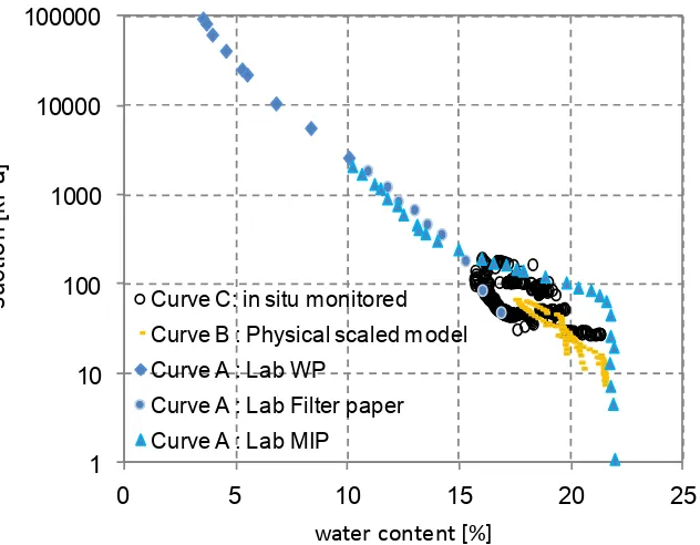
horizontal direction so that an in-situ suction-water characteristic curve (SWCC) for the 360

considered point (PR2_E2) can be obtained (curve C in Figure 8). Zielienski et al. (2011) 361

measured in the laboratory the SWCC of this glacial till with different techniques (curves A 362

in Figure 8) and the SWCC (curve B in Figure 8) in a small scale embankment made of the 363

same material. In Figure 8, all these curves are plotted. Comparing the curves, it emerges that 364

19

the laboratory and also that the boundaries of the hysteresis cycles are close. This result is 366

quite remarkable. 367

Examining the recorded temperatures of the air and ground, a clear correlation between 368

the two is found: in Figure 7b the average between the maximum and minimum daily air 369

temperature turns out to be very close to the ground temperature at 10 cm depth. Relative 370

humidity and wind speed were rather constant during the monitored period (see Figure 7c). 371 372 373 a) 374 375 b) 376 0 100 200

10-Jun-09 25-Jun-09 10-Jul-09 25-Jul-09 09-Aug-09 24-Aug-09 08-Sep-09

Su ct io n [k Pa ]

suction  EQ2

suction EQ2 0 5 10 15 20 25 30 12 14 16 18 20 22

10-Jun-09 25-Jun-09 10-Jul-09 25-Jul-09 09-Aug-09 24-Aug-09 08-Sep-09

Cu

mu

la

tiv

e  

da ily  R ai nf al

l  [

mm] G ra vi m et ric w at er co nt en t [ % ]

Pr2 10 cm Pr2 20 cm Pr2 30 cm Pr2 40 cm Pr2 60 cm Pr2 100 cm

z=10 cm z=30 cm z=20 cm z=100 cm z=60 cm z=40 cm Daily rainfall   -5.0 0.0 5.0 10.0 15.0 20.0 25.0 30.0

10-Jun-09 25-Jun-09 10-Jul-09 25-Jul-09 9-Aug-09 24-Aug-09 8-Sep-09

T em pe ra tu re [° ]

Max Temp. daily Min Temp. daily Average Daily Temp. Soil Temp. Z=15cm Mobile Average (T=10 days)

Tem

per

at

ur

e  

[⁰

C]

20 377

c)

378

Figure 7. Summer 2009 (section B): a) evolution of the gravimetric water content, suction and rainfall record;

379

b) average between the maximum and minimum daily air temperature (grey line) and ground temperature

380

measured at 10cm depth; c) relative humidity and wind speed: the thin line follows the daily variation whereas

381

the thick line is the mobile average over 10 days.

382 383

0 10 20 30 40 50 60 70

0 10 20 30 40 50 60 70 80 90 100

10-Jun-09 25-Jun-09 10-Jul-09 25-Jul-09 09-Aug-09 24-Aug-09 08-Sep-09

M

ax

im

um

s

us

ta

in

ed

w

in

d

sp

ee

d

[Km

/h

]

R

el

at

iv

e

H

um

id

ity

H

r

[%

]

21 384

Figure 8. Comparison of in situ suction - water characteristic curve (SWCC) derived from measurements taken

385

by the THP and the EQ at 25 cm depth (Curve C) with the SWCC determined from reconstituted samples

386

(Curves A, after Zielinski et al. (2011)) and in a small scale embankment model (Curve B, Zielinski et al.

387

(2011)).

388 389

In winter (see Figure 9), higher precipitations take place leading to significantly larger 390

quick increases of the ground water content, in particular at shallow depths (10 cm). The 391

same remarks as for the summer period can be made with the exception of the wind speed 392

which varies significantly more than during the summer period. 393

From the monitored data, it can be concluded that the ground water content is highly 394

sensitive to the amount of total precipitation and to the length of the dry periods whereas no 395

significant correlation to relative humidity or to the variation of wind speed was found. These 396

observations lead to state that in principle it is possible to estimate the water content in a 397

cross-section, and in turn the cross-section susceptibility to desiccation fissuring (see section 398

8), from knowledge of both ground water content at the initial time of monitoring and 399

historical rainfall records. Given the limited resources available in this project, continuous 400

measurements in time are available only in 1 section of the embankment which is too little to 401

validate a reliable correlation between historical rainfall records and water content. However 402

1 10 100 1000 10000 100000

0 5 10 15 20 25

su

ct

io

n

[kP

a]

water  content  [%] Curve C: in situ monitored

Curve B : Physical scaled model Curve A : Lab WP

22

in light of the results obtained here, we suggest that if a sufficient number of sections are 403

instrumented, a reliable correlation may be established so that meteorological data (especially 404

rainfall records) could be used to infer the amount of water content along the entire 405

embankment at any time according to the methodology presented in the next section (section 406

7) and to monitor susceptibility of the structure to desiccation fissuring (as expounded in 407

section 8). This methodology would have the advantage of not requiring periodic walk-over 408

surveys, but only the presence of a weather station nearby the structure. 409 410 411 a) 412 413 b) 414 0 5 10 15 20 25 30 12 14 16 18 20 22

12-Sep-09 27-Sep-09 12-Oct-09 27-Oct-09 11-Nov-09 26-Nov-09 11-Dec-09 26-Dec-09

Cu

mu

la

tiv

e  

da ily  R ai nf al

l  [

mm] G ra vi m et ric w at er co nt en t [ % ]

Pr2 10 cm Pr2 20 cm Pr2 30 cm

Pr2 40 cm Pr2 60 cm Pr2 100 cm Daily rainfall

z=10 cm z=30 cm z=20 cm z=100 cm z=60 cm z=40 cm   -5.0 0.0 5.0 10.0 15.0 20.0 25.0 30.0

12-Sep-09 27-Sep-09 12-Oct-09 27-Oct-09 11-Nov-09 26-Nov-09 11-Dec-09 26-Dec-09

T em pe ra tu re [° ]

Max Temp. daily Min Temp. daily

Average Daily Temp. Soil Temp. Z=15cm

Mobile Average (T=10 days)

Te

m

pe

rat

ur

e  [

⁰C]

23 415

c)

416

Figure 9. Winter 2009 (cross-section B): a) evolution of the gravimetric water content and rainfall record; b)

417

average between the maximum and minimum daily air temperature (grey line) and ground temperature

418

measured at 10cm depth; c) relative humidity and wind speed: the thin line follows the daily variation whereas

419

the thick line is the mobile average over 10 days.

420 421

6.2 Time discrete measurements of water content profiles 422

To evaluate w_{i k;} =w x z

( ) (

)

423

probe (PR) and the diviner (D) up to a depth of 1m (see Figure 10). In Figure 11a and Figure 424

11b, the evolution of the water content over time is plotted for section A and B respectively. 425

These figures were obtained by interpolating in space the values of water content measured 426

from the locations of the monitoring points (see Figure 3). The analyzed domain consists of 427

the uppermost 1 m of the cross-sections since no significant variations of water content were 428

ever observed at larger depths (see Figure 7 and Figure 9). To generate the plotted contours 429

of water content, first a mesh was created whose nodes coincide with the locations of the 430

readings taken from the PR and the D, then a post-processing FEM software, called GID 431

(GID, 2014), was employed to interpolate the values along the x and z coordinates. The 432

interpolation was repeated for measurements taken at different times (see Figure 11). From 433

these data it emerges that the water content varies significantly between the two sections. The 434

dependence of the water content on the geometrical alignment of the cross-sections, has been 435 0 10 20 30 40 50 60 70 0 10 20 30 40 50 60 70 80 90 100

12-Sep-09 27-Sep-09 12-Oct-09 27-Oct-09 11-Nov-09 26-Nov-09 11-Dec-09 26-Dec-09

M ax im um s us ta in ed w in d sp ee d [Km /h ] R el at iv e H um id ity H r [% ]

Relative Humidity [%] Maximum sustained wind speed [Km/h]

24

accounted for in deriving the function w x s z t

(

)

436

paragraph. 437

438

a) b)

439

Figure 10. Examples of profiles of the water content at different times in cross-section B: a) obtained by the

440

profile probe; b) obtained by the diviner.

441

442

a)

443

444

0 5 10 15 20 25

Moisture content [%] 100

80 60 40 20 0

D

ep

th

s

[c

m

]

Section B PROFILE PROBE PR2_W1

11/11/2008 14/11/2008 15/12/2008 26/03/2009 10/06/2009 16/07/2009 18/08/2009 08/10/2009 04/03/2010

0 5 10 15 20 25

Moisture content [%] 160

120 80 40 0

D

ep

th

[

cm

] Section B

DIVINER 2000 D_W2

25

b)

445

Figure 11. Contours of the water content at different times over a period of 1.5 years: a) in cross-section A; b)

446

in cross-section B.

447 448

7.

Extrapolation of the water content function for the entire structure

449

In the following, w x s z t

(

)

450

geotechnical suite only, secondly employing measurements of electrical conductivity taken 451

by the CMD-2 probe as well. 452

453

7.1 Derivation of the water content function from the data retrieved by the geotechnical 454

suite 455

In Figure 11, the water content of the two monitored cross-sections (A and B) is plotted. The 456

water content in any other cross-section is different due to two main factors: 457

(i) different exposure to weather conditions (e.g. sunlight, rainfall and wind) which is a

458

function of the local orientation of the considered cross-section with respect to North. 459

This factor affects the ground water content along the flanks of the embankment much 460

more than underneath the horizontal upper surface. 461

(ii) spatial variation of the geometrical, hydraulic and lithological properties of the cross

462

sections along the longitudinal coordinate s. Heterogeneities in the compaction

463

processes during construction, for example, are likely to cause a non-negligible spatial 464

variation of the hydraulic conductivity along the longitudinal direction. Concerning 465

compositional or lithological variability, this is likely to be small for the embankment 466

examined here due to the fact that it is made of homogeneous material and its young 467

age. However, in general, old earthen embankments are very often highly 468

heterogeneous comprising a mixture of several materials locally available at the time 469

26

Regarding factor (i), considering the axis of symmetry of the cross-section (axis z in Figure 471

1a), exposure to each single weather element (e.g. wind, sunrays, rainfall droplets, etc.) gives 472

rise to a variation of water content which is either anti-symmetrical or nil in the case of equal 473

exposure (e.g. no wind and vertical sunrays), but the combination of the single weather 474

elements, i.e. the sum of the anti-symmetrical variations of water content due to exposure to

475

wind, exposure to sunrays, etc., may give rise to a non-negligible symmetrical variation of 476

water content as well. The anti-symmetrical part is a function of the orientation of the cross-477

section considered whereas the symmetrical one is a function of the longitudinal coordinate s.

478

Regarding factor (ii), geometrical, hydraulic and lithological variations in the embankment 479

imply a variation of water content which in authors’ opinion is much larger along the 480

longitudinal coordinate s than within each single cross-section and therefore is mainly

481

symmetrical. In summary, the water content variation in the embankment depends on both 482

cross-section orientation and cross-section position. The latter is expressed by the 483

longitudinal distance from a reference cross section (coordinate s). To better account for the

484

variation of water content due to these geometrical factors, cross-section orientation and 485

cross-section position, it is convenient to split the water content function, w x s z t

(

)

486

parts, a symmetrical, ws, and an anti-symmetrical one, wa, with respect to the axis of

487

symmetry of the cross-section: 488

( , , , ) ( , , , ) ( , , , )

2

s w x s z t w x s z t

w x s z t = + −

and

( , , , ) ( , , , ) ( , , , )

2

a w x s z t w x s z t

w x s z t = − −

. (1)

489

To account for the influence of cross-section orientation, it is convenient to employ a 490

function

θ

491

reference direction here chosen as the geographical North (see Figure 12a). Considering 492

measurements of water content at discrete time points tk, wak

(

)

27

expressed as the weighted average of the values of water content,

494

( )

; , ( , , , )

a a

i k i k

w x z =w x s s z t t= = , recorded at t = tk in the N instrumented cross-sections:

495

( )

a a a

k k i

i

w x s z w x s z t t w x z α θ

=

= = =

∑

(2). 496

with α θ_i( ) being weight functions accounting for the anti-symmetrical water content

497

variation in the embankment. The simplest choice for α θ_i( ) _{is to consider a linear}

498

interpolation between the values of water content measured at the N instrumented sections as

499

illustrated in Figure 12c, so that: 500

[

]

[

]

(

)

(

)

[

]

(

)

(

)

[

]

1 for 1,..

0 for , 1,..

1 for 1,..

( )

1 for 1,..

i j i i i i i i i i i i i i i N

i j N

i N

i N

θ θ θ θ

θ θ _{θ θ θ}

α θ _{θ θ}

θ θ _{θ θ θ}

θ θ ≠ + + − − ⎧ = ∀ ∈ ⎪ _{= ∀ ∈} ⎪ ⎪ ₋ ⎪ − ≤ ≤ ∀ ∈ =_⎨ − ⎪ ⎪ ₋ ⎪ + ≤ ≤ ∀ ∈ − ⎪⎩ (3) 501

In general, it is advisable to instrument cross-sections forming equal angles between them so 502

that all the weight functions have the same periodicity in θ. Two sections are suggested as the

503

minimum number required for the procedure to work. 504

Analogously, with regard to the symmetrical part of the water content variation, 505

( , , , )

s s

k k

w =w x s z t t= is obtained as the weighted average of the values of water content, 506

; ( , , , )

s s

i k i k

w =w x s s z t t= = , recorded in the N instrumented cross-sections at t=tk:

507

( )

s s s

k k i

i

w x s z w x s z t t w x z β s

=

= = =

∑

(4) 508

with β_i( )s being weight functions that depend on s rather than θ. Considering again a linear

509

interpolation between the values of water content measured at the N instrumented sections as

510

illustrated in Figure 12d, β_i( )s are here defined as:

28

[

]

[

]

(

)

(

)

[

]

(

)

(

)

[

]

1 for 1,..

0 for , 1,..

1 for 1,..

( )

1 for 1,..

i j i i i i i i i i i i i i

s s i N

s s i j N

s s

s s s i N

s

s s

s s

s s s i N

s s β ≠ + + − − ⎧ = ∀ ∈ ⎪ _{= ∀ ∈} ⎪ ⎪ ₋ ⎪ − ≤ ≤ ∀ ∈ =_⎨ − ⎪ ⎪ ₋ ⎪ + ≤ ≤ ∀ ∈ − ⎪⎩ (5) 512

Unlike the case of the α_i functions, for 0≤ ≤s s₁, β1=1 whilst for s_N ≤ ≤s L, βN=1 with L

513

being the total length of the embankment. This means that for 0≤ ≤s s₁,

514

1

( , , , ) ( , , , )

s s

k k

w x s z t t= =w x s s z t t= = whilst for s_N ≤ ≤s L, s( , , , )

k

w x s z t t= =

515

( , , , )

s

N k

w x s s z t t

= = = . This is because in the regions 0≤ ≤s s₁ and s_N ≤ ≤s L, there is only

516

water content measurements are available only for 1 section so that no interpolation can be 517

carried out. Obviously in the choice of the location of the 1st and Nth cross-sections, care

518

should be taken to minimise the length of the longitudinal segments s₁−0 and L s− _N.

519

520

a) b)

521

522

c) d)

523

Figure 12. (a) plan view of the embankment layout; (b) orientation of the longitudinal axis of the embankment

524

with respect to the North; c) α weight functions against cross-section orientation; d) β weight functions against

525

longitudinal coordinate s.

526 527

x   x  

s

θ  1     θ  2     θ  Ν    

0  °    

θ  1    

360°    

α(θ)  i    

0     1    

θ  i  

s  1     s  2       s    Ν    

0     β(  s)    i    

0    

1    

s      

E  nd  of  

embankment    

29

The water content in any point of the embankment can now be obtained substituting Eqs. 528

(3) and (5) into Eq. (1): 529

( )

( )

; ;

1 1

( , , ) ( , , , ) , ( ) , ( )

i k i k

N N

a s

k k i i

i i

w x s z w x s z t t w x z α θ w x z β s

= =

= = =

∑

∑

(6)

530

In our case N=2, so that w x s z_k( , , ) is calculated as:

531

1 1 2 2

( , , ) ( , , , ) a( , , , ) ( ) a( , , , ) ( )

k k k k

w x s z =w x s z t t= =w x s s z t t= = ⋅α θ +w x s s z t t= = ⋅α θ +

532

1 1 2 2

( , , , ) ( ) ( , , , ) ( )

s s

k k

w x s s z t t= = ⋅β s +w x s s z t t= = ⋅β s

(7) 533

with 1 and 2 indicating sections A and B respectively. Note that Eq. (7) provides an analytical 534

expression for the water content in any point of the embankment at the discrete time points tk.

535

So, provided that sufficiently small space intervals between instrumented cross-sections are 536

employed and sufficiently small time intervals are used, the water content in the embankment 537

could, in principle, be monitored as accurately as desired. So, one may be tempted to 538

conclude that the use of the geotechnical suite alone is good enough for the health monitoring 539

of the embankment. However, maintenance costs of the geotechnical suite over the typical 540

lifespan of flood defence earth embankments (at least 50 years but more often 100-200 years) 541

are higher than the costs for a monitoring programme based on geophysical measurements 542

which only entail non-invasive periodic walk-over surveys. More importantly, only two 543

sections have been used here. With regards to this point, in the authors’ opinion, the proposed 544

geotechnical suite may be employed as the only monitoring method, but in order to obtain 545

accurate results, many more sections in the embankment should be monitored. If only a few 546

sections are employed to keep the monitoring costs within affordable limits, geophysical 547

probes are necessary to integrate the discrete geotechnical data with spatially continuous 548

measurements acquired along the entire embankment. Such a procedure is detailed below. 549

30

7.2 Integration of the geophysical data with the geotechnical suite 551

Herein the variable σ will be employed to represent the ground electrical conductivity which

552

is a function of both space and time, hence σ σ=

(

)

553

probes provide a measure of σ which is averaged over a prismatic volume of ground where

554

the induced electrical field is non-zero. Considering a generic cross-section of the 555

embankment, we define: 556

( )

( , , , ) , ACMD

CMD

w x s z t dxdz s t

A

σ =

∫

(8)

557

with A_CMD =b d⋅ , b being the distance between the two ends of the electromagnetic probe

558

(hence corresponding to the width of the portion of the embankment cross-section where the 559

induced electrical field is non-zero) and d the so-called effective depth, i.e. the depth of the

560

induced electromagnetic field. Note that ACMD is independent of the cross-section considered,

561

i.e. its size does not vary with s, but depends on the type of electromagnetic probe employed

562

(for this reason we called it ACMD). The effective depth is a function of the type of ground and

563

of the vertical distance from the portable device to ground level. d is an unknown that we

564

determined by trial and error selecting the value which provides the best correlation between 565

electrical conductivity and water content as illustrated later on (see Figure 14). 566

In Figure 13a, the measurements taken by the CMD-2 device at six time points along 567

the entire embankment, σ_k

( )

568

curves is approximately the same for all the times considered. Now let us introduce the 569

spatial average of σ

( )

570

( )

( , )

s L

s

s t ds t

L

σ σ

=

=

=

∫

31

with the second above score bar denoting the spatial average over the longitudinal coordinate 572

s. Then, we can introduce the normalised cross-sectional average electrical conductivity as:

573

( )

( )

_{( )}

0

,

, s t

s t

t

σ σ

σ

= (10)

574

The normalised measurements taken at times tk, i.e. σ0k =σ0

(

)

575

13b. From the figure, it emerges that the curves coincide almost perfectly. This leads to 576

consider the average of σ_0k =σ₀

(

)

577

(

)

0 0

( , )

( ) ,

( )

k k

k k _k

s t t s average s t t average

t t

σ

σ σ

σ

⎛ = ⎞

= = = _{⎜ ⎟}

=

⎝ ⎠ (11)

578

as the representative curve of the conductivity of the embankment. Note that herein the 579

underscore bar denotes time average. The measurements were taken by an operator walking 580

above the centre of the embankment horizontal upper surface. Therefore, they cannot detect 581

any conductivity variation due to different cross-section orientations, i.e. they are

582

independent of the angle θ. The time-independent function σ₀( )s can be thought of as a

583

unique identifier of the embankment expressing the variation of conductivity along the s

584

coordinate due to the variation of geometrical, hydraulic and lithological properties of cross-585

sections and to the effects of exposure to weather conditions independent of cross-section 586

orientation, i.e. cross-sectionally symmetric. On the other hand, the function σ( )t reflects the

587

temporal effect of climatic variations (e.g. rainfall, wind, temperature variations, etc.) and 588

aging on the ground conductivity. 589

32

a) b)

591

Figure 13. (a) electrical conductivity measurements along the embankments at seven different times; (b)

592

normalised values of conductivity measurements.

593 594

Now, we can split the ground conductivity function, σ

( )

595

time independent dimensionless function σ₀( )s with the space independent dimensional

596

function σ( )t :

597

0

( , )s t ( )s ( )t

σ =σ ⋅σ (12).

598

In the following it will be shown that this split is a necessary step to find a correlation 599

between water content and electrical conductivity. First, let us define the average water 600

content in the portion of the embankment cross-sections where the electromagnetic field is 601

non-zero, i.e.ACMD:

602

( )

( , , , ) , ACMD

CMD

w x s z t dxdz w s t

A

=

∫

603

Analogously to σ( , )s t , we can split w s t

( )

604

dimensionless function, w s₀

( )

605

position on the ground water content and the space independent dimensional function, w t

( )

606

which accounts for the effect of climatic variations and aging on the ground water content: 607

( )

( ) ( )

w s t =w s w t⋅ _(14).

608

( )

w t represents the spatial average of the water content on the cross-sectional area ACMD and

609

along the longitudinal coordinate s:

610

( )

1 1

0

( , , , ) ( ) ( , , , ) ( )

CMD

N N

a s

i i i i

LA i i

CMD

w x s s z t w x s s z t s dxdz

ds A

w t

L

α θ β

= =

⎡ _{= ⋅ + = ⋅} ⎤

⎢ ⎥

⎣ ⎦

=

∑

∑

∫

∫

33

To look for a correlation between the measured electrical conductivity and water content, 612

we shall consider the time dependent functions w t

( )

613

account for the strong dependency exhibited by the ground electrical conductivity on 614

temperature (Keller and Frischknecht, 1966). Recently Hayley et al., (2007) investigated this 615

dependency for a range of temperatures corresponding to our case (temperature varying 616

between 0 and 25 Celsius) on a glacial till finding a linear dependency of the type: 617

(

)

25 C T 25 1

σ σ= ⎡_⎣ − + ⎤_⎦ (16)

618

with σ being the electrical conductivity measured at the temperature T and the constant

619

C=0.02. To account for the effect of temperature on the measured electrical conductivity, we

620

expressed all the measured values relative to the same reference temperature before 621

correlating them to the water content. As shown in (Hayley et al., 2007), manipulating Eq. 622

(16), the following expression for the calculation of σ relative to the chosen reference

623

temperature is obtained: 624

(

)

(

)

1 25

1 25

ref ref

C T C T

σ =σ + −

+ − (17)

625

with σref being the value of electrical conductivity relative to the reference temperature Tref.

626

Here, we chose Tref=15 Celsius to minimise the amount of temperature compensation.

627

Employing Eq. (17), we calculated σref from the in-situ values of σ and T.

628

In Figure 14, the water content measured at the time points tk, w t t

(

)

629

the electrical conductivity measured at the same time points, σref(t t= k). It emerges that the

630

relationship between w t

( )

631

( )

( )

w t =m

σ