http://wrap.warwick.ac.uk
Original citation:
Wang, Kezhi, Chen, Yunfei, Alouini, Mohamed-Slim and Xu, Feng. (2014) BER and
optimal power allocation for amplify-and-forward relaying using pilot-aided maximum
likelihood estimation. IEEE Transactions on Communications, Volume 62 (Number 10).
pp. 3462-3475.
Permanent WRAP url:
http://wrap.warwick.ac.uk/64454
Copyright and reuse:
The Warwick Research Archive Portal (WRAP) makes this work by researchers of the
University of Warwick available open access under the following conditions. Copyright ©
and all moral rights to the version of the paper presented here belong to the individual
author(s) and/or other copyright owners. To the extent reasonable and practicable the
material made available in WRAP has been checked for eligibility before being made
available.
Copies of full items can be used for personal research or study, educational, or not-for
profit purposes without prior permission or charge. Provided that the authors, title and
full bibliographic details are credited, a hyperlink and/or URL is given for the original
metadata page and the content is not changed in any way.
Publisher’s statement:
“© 2014 IEEE. Personal use of this material is permitted. Permission from IEEE must be
obtained for all other uses, in any current or future media, including reprinting
/republishing this material for advertising or promotional purposes, creating new
collective works, for resale or redistribution to servers or lists, or reuse of any
copyrighted component of this work in other works.”
A note on versions:
The version presented here may differ from the published version or, version of record, if
you wish to cite this item you are advised to consult the publisher’s version. Please see
the ‘permanent WRAP url’ above for details on accessing the published version and note
that access may require a subscription.
BER and Optimal Power Allocation for
Amplify-and-Forward Relaying Using Pilot-Aided
Maximum Likelihood Estimation
Kezhi Wang,Student Member, IEEE,Yunfei Chen, Senior Member, IEEE,Mohamed-Slim Alouini, Fellow, IEEE,and Feng Xu
Abstract—Bit error rate (BER) and outage probability for
amplify-and-forward (AF) relaying systems with two different channel estimation methods, disintegrated channel estimation and cascaded channel estimation, using pilot-aided maximum likelihood method in slowly fading Rayleigh channels are derived. Based on the BERs, the optimal values of pilot power under the total transmitting power constraints at the source and the optimal values of pilot power under the total transmitting power constraints at the relay are obtained, separately. Moreover, the optimal power allocation between the pilot power at the source, the pilot power at the relay, the data power at the source and the data power at the relay are obtained when their total transmitting power is fixed. Numerical results show that the derived BER expressions match with the simulation results. They also show that the proposed systems with optimal power allocation outperform the conventional systems without power allocation under the same other conditions. In some cases, the gain could be as large as several dB’s in effective signal-to-noise ratio.
Index Terms—Amplify-and-forward, cascaded channel
esti-mation, disintegrated channel estiesti-mation, maximum likelihood, optimal power allocation, pilot-symbol-aided.
I. INTRODUCTION
D
UAL-HOP transmission has been commonly used in cooperative wireless communications [1]–[9]. It can be mainly categorized into: decode-and-forward (DF) and amplify-and-forward (AF) [1]. In DF systems, the relay de-codes the received signal from the source and retransmits the re-encoded signal to the destination, while in AF systems, the relay simply forwards a scaled version of the received signal to the destination with an amplification gain [1]. Depending on the nature and complexity of the AF relays, the amplification gain of AF relay can be classified as variable gain or fixed gain [3], [4]. A variable gain AF relay requires the instantaneousK. Wang and Y. Chen are with the School of Engineering, Univer-sity of Warwick, CV4 7AL Coventry, U.K. (e-mails: {Kezhi.Wang, Yun-fei.Chen}@warwick.ac.uk).
M.-S. Alouini is with the Computer, Electrical and Mathematical Sciences and Engineering (CEMSE) Division, King Abdullah University of Science and Technology (KAUST), Thuwal, Makkah Province, Saudi Arabia (e-mail: [email protected]).
F. Xu is with College of Computer and Information, Hohai University, Nanjing, China (e-mail: [email protected]).
The work of Y. Chen was supported in part by the Open Research Project of the State Key Laboratory of Industrial Control Technology, Zhejiang University, China (Grant IC14T40).
Part of this paper has been submitted for publication to the IEEE 80th Vehicular Technology Conference.
channel state information (CSI) of the first hop while a fixed gain AF relay does not need the instantaneous CSI of the first hop. Although a fixed gain relay is not expected to perform as well as a variable gain relay, it has lower energy consumption due to the saved power on the acquisition of the instantaneous CSI at the relay.
In practice, CSI is often acquired by estimation which can be performed by using either unknown or known symbols [10]. Pilot-symbol-aided system was proposed to obtain CSI using known symbols [11]. For example, linear minimum mean squared error (LMMSE) channel estimation with pilot symbols for AF relaying was studied in [7], [12], [13]. In a variable gain AF, the instantaneous CSI can be estimated both at the relay in order to determine the variable gain and at the destination for coherent demodulation, separately. This is termed as disintegrated channel estimation (DCE), as was studied in [5], [7]. Unlike a variable gain AF, in a fixed gain AF, since no CSI is required at the relay, only a cascaded channel estimation (CCE) consisting of both the source-to-relay link and the source-to-relay-to-destination link can be used to estimate CSI at the destination [5], [7]–[9], [14].
while the latter can be used in the case when the individual battery power or the individual lifetime is more important, such as moving nodes. The authors in [18] also considered similar power allocation between training and data symbols as in [16] but used outage probability measure instead. Since further integral on SNR is needed, derivations of BER and outage probability are often more difficult than that of SNR in most AF systems. Therefore, one can choose to obtain the optimal power allocation according to the application and the complexity of the AF system using the specific measure, such as SNR, outage probability or BER. Moreover, the authors in [15], [16] and [18] all considered the case when the signal experiences fast fading such that LMMSE is necessary and must be used in channel estimation. In this case, the system model is so complex such that derivations of SNR, outage probability or BER using channel estimates are very difficult, if not impossible. As a result, power allocations based on SNR, outage probability or BER often do not have closed-form in this case.
However, in many previous works [19], [20] and in high data-rate applications [21], the channel coherence time is much larger than the bit interval such that the signal only experiences slow or even block fading. In this case, since the channel gain is not time-varying, maximum likelihood (ML) estimation with a much simplified structure is more suitable to obtain the channel estimates [22]. To the best of the authors’ knowledge, none of the works in the literature have considered the optimal power allocation for AF relaying in the slowly fading channel using ML esimation.
In this work, we consider the optimal power allocation for AF relaying system in slowly fading Rayleigh channel using pilot-symbol-aided ML channel estimation. Our contributions can be summarized as follows:
• We first introduce the pilot-symbol-aided ML estimation method for both DCE and CCE. For DCE, we consider the case when the fading gain is estimated at the relay as well as the case when the fading gain is estimated at both the relay and destination, separately. For CCE, we only consider the case when the fading gain is estimated at the destination. Based on these, the outage probability of AF relaying for DCE and CCE is derived for variable and fixed gains, respectively.
• We then derive the the general form of the bit error rate (BER) for high order modulations with DCE and CCE. We provide two kinds of closed-form approximations for DCE with different complexity and accuracy while we provide closed-form approximations for CCE with two kinds of am-plification factors.
• More importantly, using the BER expressions of both DCE and CCE, the optimal values of pilot power under the total transmitting power constraint at the source and at the relay are obtained, separately. This is the case when the source, relay or destination are battery-limited moving nodes. Moreover, the optimal power allocation between the pilot power at the source, the pilot power at the relay, the data power at the source and the data power at the relay are obtained when their total transmitting power are fixed. This is the case when the source, relay and destination are fixed nodes that can be charged.
II. SYSTEM MODEL ANDPILOT-AIDEDMLESTIMATION
Consider an AF cooperative system with one source, one destination and one relay. There is no direct link between the source and the destination. In the first time slot, the source transmits the signal to the relay such that the received signal at the relay can be expressed as
u(t) =√Ed h1s(t) +n1(t) (1)
whereh1 is the complex fading gain in the channel between
the source and the relay,Edis the transmitted signal energy per
data symbol,s(t)is the transmitted data symbol with the unit power such thatE{|s(t)|2}= 1,E{·}denotes the expectation operator, andn1is the complex additive white Gaussian noise
(AWGN) in the channel between the source and the relay with noise powerN1.
In the second time slot, the received signal at the relay is amplified and forwarded such that the received signal at the destination is
y(t) =G h2u(t) +n2(t) (2)
whereh2 is the complex fading gain in the channel between
the relay and the destination, n2 is the complex AWGN in
the channel between the relay and the destination with noise powerN2, andGis the amplification factor. Assume that all
the links experience Rayleigh fading with E {
|h1| 2}
= Ω1
andE {
|h2| 2}
= Ω2. Assume thatris the path-loss exponent
and thatd1 and d2 are the distances between the source and
the relay, the relay and the destination, respectively. Therefore, one has Ω1=Ld−1r and Ω2 =Ld−2r, where L is a constant
that takes antenna gains and other power factors into account. We also assume that all nodes have similar transmitter/receiver settings such thatL is the same for all hops.
Define the instantaneous signal-to-noise ratio (SNR) be-tween source and relay, and bebe-tween relay and destination as
γ1 =Ed |h1|2/N1 andγ2 =Es |h2|2/N2, respectively, and
the average SNR as γ¯1 =Ed Ω1/N1 and ¯γ2 = Es Ω2/N2,
respectively, where Es is the transmitted energy per data
symbol at the relay that is included in G. Therefore, the probability density functions (PDFs) of γ1 and γ2 are given
byf(γ1) = γ1¯
1e
−γ1 ¯
γ1 andf(γ2) = 1
¯
γ2e
−γ2 ¯
γ2, respectively [10]. Consider the case whenW1 pilot symbols each with
trans-mitted energyEw1 are inserted beforeD data symbols at the source, giving a frame of W1+D symbols. At the relay, in
DCE,W2pilot symbols each with the transmitted energyEw2 are inserted into the frame received from the source, while in CCE, the same pilot symbolsW1from the source are amplified
and forwarded to the destination with transmitted energyEw2 such that no additional pilots are inserted at the relay. We still use the notationW2to denote the number of pilot symbols at
the relay for CCE but W2=W1 in this case.
the random interferences that occur in the pilot or data transmission periods separately. Also, assume block fading channels such that the fading gains remain the same during the whole frame.
Let PT,P1,P2,Pd,Ps,Pw1 andPw2 be the total power, the total power at the source, the total power at the relay, the total data power at the source, the total data power at the relay, the total pilot power at the source and the total pilot power at the relay, respectively. Therefore, one has PT =P1+P2, P1 =Pd+Pw1, P2 =Ps+Pw2,Pd =D Ed,Ps=D Es,
Pw1 =W1Ew1,Pw2 =W2Ew2 in both DCE and CCE. Let
H1=D+W1,H2=D+W2andH =H1+H2. Also, letP1∗, P2∗,Pd∗,Ps∗,Pw∗1 andPw∗2 be the optimal total power at the source, the optimal total power at the relay, the optimal data power at the source, the optimal data power at the relay, the optimal pilot power at the source and the optimal pilot power at the relay, respectively. Note that in this paper we consider the optimal power for the whole frame in terms of Pd∗, Ps∗,
Pw∗1 andP
∗
w2, instead of the optimal power for one symbol as in [18], [23]. In this case, one can adjust either the number of symbols or the power of one symbol to achieve this under the total power constraints for specific application, which is more general and also more flexible than the optimal power for one symbol. Note also that this paper considers the case when the signal experiences block fading channel such that the channel gain keeps the same in one frame. Therefore, pilot symbols can be either interleaved with the data symbols or inserted as a preamble before the data symbols, as they do not need to sample the fading process. In fast fading channels, since the fading process is time-varying, these two schemes may be different and the interleaving rate will depend on the fading rate. In the following, we will introduce the amplification factor and ML estimation for both DCE and CCE.
A. DCE
In DCE, the amplification factorGis defined as [1]
ˆ
G2var= Es
Edˆh1 2
+N1 .
(3)
In this case, the relay and the destination estimateh1 andh2,
separately. Let h1 =x1+iy1, wherex1, y1 are independent
and identically distributed random variables with zero mean and variance Ω1/2. Assume that ˆh1 = ˆx1 + iyˆ1, where
ˆ
h1, xˆ1, yˆ1 are estimates of h1, x1, y1 respectively. Using
the pilot-symbol-aided ML estimation [22], one can have ˆ
x1 ∼ N(x1,
Nw1
2Ew1W1) and yˆ1 ∼ N(y1,
Nw1
2Ew1W1), where N{·,·}denotes the normal distribution. Therefore, one can get the PDF of|hˆ1|as
f|ˆh
1|(x) = 2xe−
x2Ew1W1
Nw1+Ew1Ω1W1Ew 1W1
Nw1+Ew1Ω1W1
, x >0. (4)
Similarly, one can get the PDF of |ˆh2|as
f|ˆh2|(x) = 2xe−
x2Ew2W2 Nw2+Ew2Ω2W2E
w2W2
Nw2+Ew2Ω2W2
, x >0. (5)
Define the estimated instantaneous SNR in the channel be-tween the source and the relay, and that bebe-tween the relay and the destination as ˆγ1=Ed |ˆh1|2/N1 andγˆ2 =Es|ˆh2|2/N2,
or γˆ1 = PDd |ˆh1|2/N1 and γˆ2 = PDs |ˆh2|2/N2, respectively.
Therefore, one can calculate the estimated average SNR as ¯
ˆ
γ1 = ¯γ1+γε1 and γˆ¯2 = ¯γ2+γε2, respectively, where γε1 andγε2 are defined as the statistics of the channel estimation errors between source and relay, and between relay and destination, respectively, with the values of γε1 =
EdNw1
N1Ew1W1 andγε2 =
EsNw2
N2Ew2W2. Thus, the PDF ofγˆ1andˆγ2can be given byf( ˆγ1) = γ1¯ˆ
1e
−γˆ1 ¯ ˆ
γ1 andf( ˆγ 2) = γ1¯ˆ
2e
−γˆ2 ¯ ˆ
γ2, respectively.
B. CCE
In CCE, the amplification factorGfor the data symbols at the relay can be written as [3]
G2d
f ix1 =E
[ Es
Edh21+N1 ]
=
Ese
N1 EdΩ1Γ
(
0, N1
EdΩ1
)
EdΩ1
(6)
or [24]
G2df ix2 =
Es
E[Edh21+N1]
= Es
EdΩ1+N1
. (7)
Similarly, the amplification factor for the pilot symbols at the relay is [3]
G2w
f ix1 =E
[
Ew2
Ew1h
2 1+Nw1
]
=
Ew2e
Nw1 Ew1Ω1Γ
(
0, Nw1
Ew1Ω1
)
Ew1Ω1
(8) or [24]
G2w f ix2 =
Ew2
E[Ew1h
2 1+Nw1]
= Ew2
Ew1Ω1+Nw1
. (9)
Instead of estimatingh1andh2separately at the relay and
at the destination as in DCE, we estimate the product of h1
andh2at the destination in CCE. In this case, the relay uses a
fixed gain which remains constant and no estimator is needed at the relay to simplify the structure of the relay. On the other hand, in DCE, extra energy is consumed to estimate the instantaneous CSI forGˆvar, although DCE has a slightly
better performance than CCE in some regions [4]. Define the instantaneous equivalent channel gain between the source and the destination as H. Then the received pilot symbol at destination can be written as
y=√Ew1H Gwf ix1 s+nw (10)
whereH =h1h2 andnw=Gwf ix1 h2nw1+nw2. The PDF of |H| is given as [25]
f|H|(x) =
4xK0 (
2
√
x2
Ω1Ω2
)
Ω1Ω2
, x >0. (11)
Define the estimated instantaneous equivalent channel gain between the source and the destination as Hˆ. Also, nw in
and following the same process as in DCE, one can get the PDF of |Hˆ|as
f|Hˆ|(x) =
4xK0 (
2
√
x2
Ω )
Ω , x >0
(12)
where Ω = Ω1Ω2 + Ωε, Ωε =
Nw2+G 2
wfix1Nw1Ω2
Ew1G2wfix1W1 can be considered as the variance of the channel estimation error. The PDF of |Hˆ| using Gwf ix2 can be obtained in the same way.
III. BERAND OPTIMAL POWER ALLOCATION INDCE
In this section, we first derive the outage probability and BER of AF using a variable gain in DCE and then study the optimal power allocation under the total transmitting power constraint. In the first subsection, we consider the case when the relay estimatesh1 and the destination has perfect
knowl-edge of h2. This is the case for mobile relays with limited
complexity and power but fixed destination with enough power for accurate h2. It serves as a benchmark for the case when
both are estimated. In the second subsection, we consider the case when both the relay estimates h1 and the destination
estimatesh2, separately.
A. When h1 is estimated at the relay
1) Outage probability and BER: The received signal at the destination can be written by omitting the time indexes as
y=√Edh1h2Gˆvar s+ ˆGvarh2n1+n2. (13)
Since ˆh1 is the estimate of h1 withˆh1 =h1+ε1, whereε1
is the channel estimation error, one has
y=√Ed(ˆh1−ε1)h2Gˆvar s+ ˆGvar h2n1+n2. (14)
After simplification, one has
y=√Edˆh1h2Gˆvars−
√
Ed ε1h2Gˆvars+ ˆGvar h2n1
+n2.
(15) The end-to-end SNR can be derived from (15) as
γend1 =
γ2γˆ1 γ2+ ˆγ1+ 1 +γε1 γ2
(16)
where E{|ε1|2} =
Nw1
Ew1W1 and E{|s|
2} = 1 are assumed,
and other symbols are defined as before. The value of ε1 is
considered as random disturbance, similar to noise. That is whyε1does not appear in (16) and only its statistics do. It is
derived in Appendix A that the outage probability using the end-to-end SNR in (16) is
Fγend1(γth) = 1−
2e−
γth(γε1γ¯2 +γ¯ˆ1 +¯γ2)
¯ ˆ
γ1 ¯γ2 K1
√ 2
¯
γ2γ¯ˆ1
γth(γε1γth+γth+1) √
¯
γ2¯ˆγ1
γth(γε1γth+γth+1)
,
(17)
whereKv(·) is thevth order modified Bessel function of the
second kind [26]. Using (17), the BER can be calculated as [27]
Pe=
a
2
√ b
2π ∫ ∞
0 e−2bx
√
x Fγend1(x)dx (18) where a and b are modulation-specific constants including (a, b) = (1,1) for BFSK, (a, b) = (1,2) for BPSK and (a, b) = (2MM−1,M26−1)for M-PAM. Also, the BER
expres-sion in (18) is a good approximation to the BER of some higher order modulations, such as(a, b) = (2,2sin2(π/M))
for M-PSK.
The BER in (18) can be approximated in two ways. First, one can approximate the BER as
Pe≈
1 2a
(
1−
√ b √
b+ 2β2 )
(19)
whereβ2= ¯ ˆ
γ1+¯γ2γε1+¯γ2
¯ ˆ
γ1¯γ2 . Proof: See AppendixB.
Second, one can get the approximate BER as (20), whereβ1= 2√√γε1+1
¯ ˆ
γ1¯γ2
,κν(·)is the complete elliptic integral of theνth kind
defined in [26] withκ1(k) = ∫π/2
0
dx
√
1−ksin2(x) andκ2(k) =
∫π/2 0
√
1−ksin2(x)dx. Proof: See AppendixC.
2) Optimal power allocation: Since we consider the case when the relay estimates h1 and the destination has perfect
knowledge ofh2, we only derive the optimal power allocation
between Pd and Pw1 under the fixed total power P1 at the source. Since (19) is simpler than both (18) and (20), we use (19) to derive the optimal allocation. One can observe that minimizing (19) is equivalent to minimizingβ2. Inserting Ed = PDd,Ew1 =
Pw1
W1 andPd =P1−Pw1 into β2, one can get
β2=
DPw1N1
(P1−Pw1)(Pw1Ω1+Nw1) + N2
EsΩ2
+ Nw1
Pw1Ω1+Nw1
.
(21) Differentiating (21) with respect to Pw1, equating it to zero and solving the equation, the optimal value of Pw1 can be found as
Pw∗1= µ1−P1Nw1Ω1
DN1Ω1−Nw1Ω1
(22)
where µ1 = (−D2P1N12Nw1Ω1 + DP
2
1N1Nw1Ω
2 1 + DP1N1Nw21Ω1)
1/2. Then, by using P∗
w1 of (22), the optimal value of Pd can be found as Pd∗ = P1−Pw∗1. One can see from (22) that the optimal pilot power at the source increases when Ω1 increases, or when the distance between the source
and the relay decreases, asΩ1=Ld−1r.
B. When bothh1 andh2are estimated at the relay and at the
destination, separately
1) Outage probability and BER: In this case, the received signal at destination can be written as
Pe≈
1 2a
√ b
√ β1
(
(b+ 2(β1+β2))κ1 (
−b−2β1+2β2
4β1
)
−2(b+ 2β2)κ2 (
−b−2β1+2β2
4β1
))
(b−2β1+ 2β2)(b+ 2(β1+β2))
+√1
b
(20)
Letˆh1,ˆh2 be the estimates ofh1,h2, respectively, withˆh1= ε1+h1 and ˆh2 =ε2+h2 where ε1 and ε2 are the channel
estimation errors. Thus,
y=√Ed(ˆh1−ε1) (ˆh2−ε2) ˆGvars+ ˆGvar (ˆh2−ε2)n1
+n2.
(24) The end-to-end SNR in this case can be written as
γend2=
ˆ
γ2γˆ1
ˆ
γ2γε1+ ˆγ1γε2+γε1γε2+ ˆγ2+ ˆγ1+ 1 +γε2 (25) whereE{|s|2}= 1,E{|ε
1|2}=
Nw1
Ew1W1,E{|ε2|
2}= Nw2
Ew2W2 and other symbols are defined as before. It is derived in AppendixDthat the outage probability of the end-to-end SNR in (25) is
Fγend2(γth) = 1−2e
−γth(γε1γ¯ˆ2 +γε2γ¯ˆ1 +γ¯ˆ1 +¯ˆγ2 ) ¯
ˆ
γ1γ¯ˆ2
× K1
√ 2
¯ ˆ
γ1γ¯ˆ2
γth(γε1γth+γth+(γε1+1)γε2(γth+1)+1)
√ ¯
ˆ
γ1γ¯ˆ2
γth((γε1+1)γε2(γth+1)+γε1γth+γth+1) .
(26)
Similarly, the BER is given by
Pe=
a
2
√ b
2π ∫ ∞
0 e−b2x
√
x Fγend2(x)dx. (27) Using the same approximations as before, the BER in (27) can be approximated as
Pe≈
1 2a
(
1−
√ b √
b+ 2β4 )
(28)
or (29), where β3 =
2√(γε√1+1)(γε2+1) ¯
ˆ
γ1γ¯ˆ2
and β4 =
¯ ˆ
γ1γε2+¯γˆ1+¯ˆγ2γε1+¯ˆγ2
¯ ˆ
γ1γ¯ˆ2 .
2) Optimal power allocation: In the first part of this subsection, we consider the optimal allocation between Pd
and Pw1 under fixed P1, and the optimal allocation between
Ps and Pw2 under fixed P2, separately. In the second part, we consider the optimal allocation betweenPd,Ps,Pw1,Pw2 under the fixed total power PT. Similarly, we useβ4 in (28)
to derive the optimal power allocation below.
Firstly, by inserting Ed = PDd, Es = PDs, Ew1 =
Pw1
W1,
Ew2 =
Pw2
W2,Pd=P1−Pw1 andPs=P2−Pw2 intoβ4, one can get
β4=
DPw1N1+Nw1(P1−Pw1)
Nw1(P1−Pw1) +Pw1Ω1(P1−Pw1) + DPw2N2+Nw2(P2−Pw2)
Nw2(P2−Pw2) +Pw2Ω2(P2−Pw2)
.
(30)
Differentiating (30) with respect to Pw1, Pw2 and equating them to zero, respectively, the optimal values ofPw1 andPw2
can be found as
Pw∗
1 =
µ1−P1Nw1Ω1
DN1Ω1−Nw1Ω1
(31)
and
Pw∗2 = µ2−P2Nw2Ω2
DN2Ω2−Nw2Ω2
(32)
respectively, where µ2 = (−D2P2N22Nw2Ω2 +
DP2
2N2Nw2Ω
2
2 + DP2N2Nw22Ω2)
1/2. Then, by using Pw∗
1 of (31) and P
∗
w2 of (32), the optimal values of Pd and
Ps can be found as Pd∗ = P1−Pw∗1 and P
∗
s = P2−Pw∗2, respectively.
Secondly, inserting Pw∗1,Pw∗2,Pd∗,Ps∗ and P2 =PT −P1
intoβ4 in (30), differentiating it with respect toP1, equating
it to zero and solving the equation, one can get
α2
10(α4(α3−2Nw1Ω1α4)−α2α3)
α1α22α4
+
α2 7 (
2Ω2α26(DN2α8+Nw2α5) +α9(α5(α6−α8) +α6α8)
)
α2 5α6α28
+α
2
10(α3−2DN1Ω1α4) α2
1α2
= 0
(33) whereα1=α4−DP1N1Ω1,α2=DN1Nw1−P1Nw1Ω1−
N2
w1+α4,α3=DP1N1Nw1Ω
2
1−DN1Nw1Ω1(DN1−P1Ω1−
Nw1), α4 = [−DP1N1Nw1Ω1(DN1 −P1Ω1 −Nw1)]
1/2, α5 = α6−DN2Ω2(PT −P1), α6 = [−DN2Nw2Ω2(PT −
P1)(DN2−Ω2(PT −P1)−Nw2)]
1/2, α
7 = Nw2 −DN2,
α8 = DN2Nw2 −Nw2Ω2(PT −P1)−N
2
w2 +α6, α9 =
DN2Nw2Ω2(DN2−Ω2(PT−P1)−Nw2)−DN2Nw2Ω
2 2(PT−
P1) and α10 = Nw1 − DN1. Note that (33) does not lead to a closed-form expression for the optimal value of
P1∗ but can be calculated numerically by using commonly adopted mathematical software packages, such as MATLAB, MATHEMATICA and MAPLE. With the optimal value ofP1∗
obtained from (33), one can easily calculate the optimal value of P2∗ and the following optimal values of Pd∗, Ps∗, Pw∗1 and
Pw∗2 under the fixed total power PT. Note that the optimal
value of P1∗ obtained from (33) is the exact optimal value for the total power at the source. In the following, we give a simpler approximate closed-form value for P1∗ under high SNR conditions. When the SNR is high, β4 in (30) can be
approximated as
β5≈
DPw1N1+Nw1(P1−Pw1)
Pw1Ω1(P1−Pw1) +DPw2N2+Nw2(P2−Pw2)
Pw2Ω2(P2−Pw2)
.
(34)
Differentiating (34) with respect to Pw1, Pw2 and equating them to zero, respectively, the optimal values ofPw1 andPw2 can also be found as
Pw∗
1=
P1µ5 µ3
Pe≈
1 2a
√ b
√ β3
(
(b+ 2(β3+β4))κ1 (
−b−2β3+2β4
4β3
)
−2(b+ 2β4)κ2 (
−b−2β3+2β4
4β3
))
(b−2β3+ 2β4)(b+ 2(β3+β4))
+√1
b
(29)
and
Pw∗2 =
P2µ6 µ4
(36)
respectively, whereµ3=DN1−Nw1, µ4=DN2−Pw2, µ5=
√
DN1Nw1−Nw1, µ6=
√
DN2Nw2−Nw2. By using Pw∗1 in (35) andPw∗
2 in (36), the optimal values ofPd andPscan be found asPd∗=P1−Pw∗1 andP
∗
s =P2−Pw∗2, respectively. One can see from (35) and (36) that the optimal pilot powers at the source and at the relay increase with the increases of
P1andP2, respectively. Then, by insertingPw∗1,P
∗
w2,P
∗
d,Ps∗
andP2=PT−P1 into β4 in (30) and differentiating it with
respect to P1, and equating it to zero, one can get √
Ω1µ3µ5(µ4−µ6)(DN1µ5+Nw1(µ3−µ5)) Ω2µ4µ6(µ3−µ5)(DN2µ6+Nw2(µ4−µ6)) = P1Ω1µ5+Nw1µ3
(PT −P1)Ω2µ6+Nw2µ4
.
(37)
Letting µ7 = √
Ω1µ3µ5(µ4−µ6)(DN1µ5+Nw1(µ3−µ5))
Ω2µ4µ6(µ3−µ5)(DN2µ6+Nw2(µ4−µ6)), one can get
P1∗=PTΩ2µ6µ7−Nw1µ3+Nw2µ4µ7 Ω1µ5+ Ω2µ6µ7
. (38)
With the value ofP1∗obtained in (38), one can easily calculate the value of P2∗ and the following optimal values ofPd∗,Ps∗,
Pw∗
1 andP
∗
w2 under the fixed total powerPT. Note that from our simulations, it is found that the values ofPw∗
1 in (35) and
Pw∗
2 in (36) are nearly the same as the values ofP
∗
w1 in (31) and Pw∗2 in (32), respectively. Thus (35) and (36) are very good approximations. Also, the optimal value ofP1∗ obtained from (38) is nearly the same as the value obtained in equation (33), but (38) gives a closed-form expression ofP1∗, which is preferable in some applications.
IV. BERAND OPTIMAL PILOT POWER ALLOCATION IN CCE
In this section, we first derive the outage probability and BER of AF using a fixed gain in CCE, and then derive the optimal power under the total transmit power constraints. In the first subsection, we use Gdf ix1 andGwf ix1, while in the second subsection, we use Gdf ix2 andGwf ix2.
A. Using Gdf ix1 and Gwf ix1
1) Outage probability and BER: In this case, the received signal at the destination is
y=√Edh1h2Gdf ix1 s+Gdf ix1 h2n1+n2. (39) Assuming H = h1 h2 and n = Gdf ix1 h2 n1+n2, (39) becomes
y=√EdH Gdf ix1 s+n. (40)
LetHˆ be the estimate ofH, andHˆ =H+ε, whereεdenotes the channel estimation error. One has
y=√EdH Gˆ df ix1 s−
√
Edε Gdf ix1 s+n. (41) The end-to-end SNR can be derived from (41) as
γf ix=
EdHˆ2G2df ix1
Ed ΩεG2df ix1+N
(42)
whereN =G2
df ix1N1Ω2+N2andE{|s|
2}= 1. It is derived
in Appendix E that the outage probability of the end-to-end SNR in (42) can be written as
Fγf ix(γth) = 1−2 v u u
tγth(EdΩεG2df ix
1 +N)
EdG2df ix1 Ω
×K1 2
v u u
tγth(EdΩεG2df ix1+N)
EdG2df ix1 Ω
.
(43)
Usingγf ix in (42), the BER is derived as
Pe=
∫ ∞
0 aQ
v u u
tb Ed Hˆ2G2df ix
1
EdΩεG2df ix1 +N
fHˆ( ˆH)dH.ˆ (44)
One can use the PDF ofHˆ in (12) with [26, (6.62)] to solve the integral as
Pe=
aG22,,23 (
2(EdΩεG2dfix
1
+N)
bEdG2dfix
1
Ω | 1 2,1
1,1,0
)
2√π
(45)
where a, b are defined as in (18) and G22,,23(·) denotes the Meijer’s G−function [26]. Using the approximationΓ[0, x]≈
−e−x
−x [26] in (6) and (8), one can have G
2
df ix1 ≈
Es
N1 and G2
wf ix1 ≈
Ew2
Nw1
. Therefore, the BER in (45) can be approximated as (46).
2) Optimal power allocation: Denotingβ6 as
β6= [2(EdEsNw1(Nw2+Ew2Ω2) +Ew1Ew2N1 (N2+EsΩ2)W1)]/[bEdEs(Nw1(Nw2+Ew2Ω2)
+Ew1Ew2Ω1Ω2W1)],
(47)
one can observe that minimizing Pe in (46) is equivalent to
minimizingβ6. However,β6in (47) is a complicated function
that does not lead to any closed-form expressions for the optimal power allocation. Therefore, we simplify the equations for high SNR as
β6≈
2EdNw1+ 2Ew1N1W1
bEdEw1Ω1W1+bEdNw1
. (48)
Pe≈
aG22,,23 (
2(EdEsNw1(Nw2+Ew2Ω2)+Ew1Ew2N1(N2+EsΩ2)W1)
bEdEs(Nw1(Nw2+Ew2Ω2)+Ew1Ew2Ω1Ω2W1) |
1 2,1
1,1,0
)
2√π .
(46)
which will be justified in Section V. By inserting Ed = PDd,
Ew1 =
Pw1
W1 and Pd = P1 −Pw1 into β6 in (48) and differentiating it with respect toPw1, then equating it to zero, one can get the optimal value of Pw1 as
Pw∗1 = µ1−P1Nw1Ω1
DN1Ω1−Nw1Ω1
. (49)
Then, the optimal value ofPdcan be found asPd∗=P1−Pw∗1. One can see that (48) does not includeEsandEw2 due to high SNR approximation. Therefore, we use β6 of (47) to get the
optimal values ofPsandPw2. By insertingEs=
Ps
D,Ew2=
Pw2
W2 andPs=P2−Pw2 intoβ6 of (47) and differentiating it with respect toPw2, then equating it to zero, one can get the optimal value ofPw2 as
Pw∗2 = [µ8+P2Nw1Nw2Ω2W1(DN1−PdΩ1)]/[D
2N 1N2
Ω2(Pw∗1Ω1+Nw1) +Nw1Nw2Ω2W1(DN1−PdΩ1)] (50) where µ8 = [D2P2N1N2Nw1Nw2Ω2W1((Pw∗1Ω1 +
Nw1)(−D
2N
1N2 + D(−P2)N1Ω2 + P2PdΩ1Ω2) + Nw1Nw2W1(PdΩ1−DN1))]
1/2. Then, the optimal value of Pscan be found as Ps∗=P2−Pw∗2. In this case, the optimal power allocation between Pd, Ps, Pw1, Pw2 under the fixed total power PT can be obtained by first inserting Pw∗1,P
∗
w2,
Pd∗,Ps∗ andP2=PT−P1 intoβ6in (47) and differentiating
it with respect to P1, then equating it to zero. However, the
results are not presented here since it is very complicated and do not provide much insight to the performance analysis, although it can be easily extracted using the well-known mathematical software packages. We will provide the optimal power allocation between Pd, Ps, Pw1, Pw2 under fixed PT for the case when Gdf ix2 in (7) andGwf ix2 in (9) are used in the next subsection.
B. Using Gdf ix2 and Gwf ix2
1) Outage probability and BER: In this case, usingGdf ix2 in (7) andGwf ix2 in (9), the outage probability can be easily obtained by replacingGdf ix1 andGwf ix1 in (43) withGdf ix2
andGwf ix2, respectively. Also, the BER expressionPein (44)
can be solved as (51), wherea,bare defined as in (18). Using the approximations of G2
df ix2 ≈
Es
EdΩ1 and G
2
wf ix2 ≈
Ew2
Ew1Ω1 in high SNR, the BER in (51) can be approximated as (52).
2) Optimal power allocation: Denotingβ7 as
β7= [2(Ew1Ew2W1(EdN2Ω1+EsN1Ω2) +EdEs (Ew1Nw2Ω1+Ew2Nw1Ω2))]/[bEdEs(Ew1Ω1(Ew2Ω2W1
+Nw2) +Ew2Nw1Ω2)].
(53) One can observe that minimizing Pe in (52) is equivalent to
minimizingβ7. However,β7in (53) is a complicated function
that does not lead to any closed-form expressions for optimal
power allocation. Therefore, we simplifyβ7 for high SNR as
β7≈[2EdEw1Ew2N2Ω1W1+ 2EdEw1EsNw2Ω1+ 2EdEw2EsNw1Ω2+ 2Ew1Ew2EsN1Ω2W1]/[bEdEw1Ew2
EsΩ1Ω2W1+bEdEw2EsNw1Ω2].
(54) Firstly, by insertingEd= PDd,Es=PDs,Ew1 =
Pw1
W1,Ew2 =
Pw2
W2,Ps=P2−Pw2 andPd=P1−Pw1 intoβ7in (54) and differentiating it with respect to Pw1 and Pw2, then equating them to zero, respectively, one can get the optimal value of
Pw2 as
Pw∗
2=
P2 √
N2DNw2−P2Nw2
DN2−Nw2
(55)
and the optimal value ofPw1 as
Pw∗
1 =
µ9+P1Nw1Ω1(DPw∗2N2+Ps(Nw2−Pw∗2Ω2)) Ω1(DPw∗2(PsN1Ω2+N2Nw1) +PsNw1(Nw2−Pw∗2Ω2))
(56) where µ9 = (−DP1Pw∗2PsN1Nw1Ω1Ω2(DPw∗2(N2(P1Ω1+
Nw1) +PsN1Ω2) +Ps(P1Ω1+Nw1)(Nw2 −Pw∗2Ω2)))
1/2.
Then, by usingPw∗
1 in (56) andP
∗
w2 in (55), the optimal values of Pd and Ps can be found as Pd∗ = P1−Pw∗1 and P
∗
s =
P2−Pw∗2, respectively.
Secondly, in order to get the optimal power allocation between Pd, Ps,Pw1, Pw2 under fixed PT,Pw∗1 in (56) and
Pw∗2 in (55) must be approximated to obtain simpler forms. Following the same process as that in Section III.B, β7 in
(54) can be approximated as
β8≈
2
( DPw1
(
N1
P1−Pw1
+ N2Ω1
P2Ω2−Pw2Ω2
)
+Pw1Nw2Ω1
Pw2Ω2 +Nw1
)
b(Pw1Ω1+Nw1)
.
(57) Differentiating β8 in (57) with respect to Pw1, Pw2 and equating them to zero, respectively, the approximate optimal values of Pw1 andPw2 can be found as
Pw∗
1=
P1µ5 µ3
(58)
and
Pw∗2= P2µ6
µ4
(59)
respectively. One can see thatPw∗
1 and P
∗
w2 in (58) and (59) are the same as the optimal values obtained in Section III.Bfor DCE. By usingPw∗
1 in (58) andP
∗
w2 in (59), the approximate optimal values ofPd andPscan be found asPd∗=P1−Pw∗1 and Ps∗ = P2 −Pw∗2 respectively. Then, by inserting those approximate Pw∗1, Pw∗2, Pd∗, Ps∗ and P2 = PT −P1 into β8
and differentiating it with respect to P1, then equating it to
zero, one can get
P1∗=
√ P2
Tµ11µ12−µ10µ11+µ10µ12−PTµ12 µ11−µ12
Pe=
aG22,,23 (
2EdEs(Ew1Nw2Ω1+Nw1(Nw2+Ew2Ω2))+2Ew1Ew2(EdN2Ω1+N1(N2+EsΩ2))W1
bEdEs(Nw1(Nw2+Ew2Ω2)+Ew1Ω1(Nw2+Ew2Ω2W1)) |
1 2,1
1,1,0
)
2√π
(51)
Pe=
aG22,,23 (
2(EdEs(Ew1Nw2Ω1+Ew2Nw1Ω2)+Ew1Ew2(EdN2Ω1+EsN1Ω2)W1)
bEdEs(Ew2Nw1Ω2+Ew1Ω1(Nw2+Ew2Ω2W1)) |
1 2,1
1,1,0
)
2√π .
(52)
whereµ10=PTNw1µ3µ4(µ3−µ5)(DN2µ6+Nw2(µ4−µ6)),
µ11= Ω1µ4µ5(µ3−µ5)(DN2µ6+Nw2(µ4−µ6))andµ12= Ω2µ3µ6(µ4−µ6)(DN1µ5+Nw1(µ3−µ5)). With the value of P1∗ obtained in (60), one can easily calculate the value of
P2∗and the following optimal values ofPd∗,Ps∗,Pw∗
1 andP
∗
w2 under the fixed total power PT. Similarly, these approximate
optimal values obtained here are nearly the same with the exact values from our simulations, as will be shown later.
V. NUMERICAL RESULTS AND DISCUSSION
In this section, numerical results are presented to illustrate and verify our theoretical analysis. In the first subsection, the BER expressions of AF using a variable gain in DCE and using two types of fixed gain in CCE are examined. In the simulation, 106 Monte-Carlo simulation runs are used.
Each run has a different channel realization but the same bit. There is no iteration. In the second subsection, the BER performances with optimal power values are compared with the conventional system without optimal power allocation. We use (a, b) = (1,2) for BPSK, (a, b) = (1.5,0.4) for 4-PAM and (a, b) = (2,1) for the approximation of QPSK. Also, we use L = 1, the path-loss exponent r = 3, W1 = 5, W2 = 5 and D = 45 in the examples below. Note that the
total pilot power and the total data power, not the individual symbol powers, are optimized in this paper. As a result, one can either fix the individual symbol powers and optimize the symbol numbers, or fix the symbol numbers and optimize the individual symbol powers, or both. In the examples, we fix the symbol numbers and optimize the individual symbol powers. Other values of W1,W2 andD or other methods of
optimization can be examined in a similar way. They have the same effects as it is the total power that determines the system performance and that is optimized. Denote the BER expressions in (18), (27), (45) or (51) as “Exact”, the BER expressions in (19), (28), (46) or (52) as “Approximation-1” and BER expressions in (20) or (29) as “Approximation-2”. Exact BER expressions in (18) and (27) in the form of one-dimensional integral are calculated numerically by using the “NIntegrate” method in MATHEMATICA software package while other BER expressions in closed-form are calculated directly.
A. Validation of BER Expressions
Fig. 1 - Fig. 3 show the BERs vs.¯γ1, where we setd1= 1, d2= 1,N1= 1,N2= 1,Nw1= 1,Nw2 = 1,γε1 =−10dB and γ¯1 = 2¯γ2. One can see from Fig. 1 - Fig. 3 that BPSK
gives the best BER performance while 4-PAM gives the worst
BER performance. But QPSK and 4-PAM can transmit twice the data rate in a given bandwidth compared to BPSK. Thus it is a tradeoff between reliability and rate.
Fig. 1 (a) compares the BERs obtained by simulation, “Ex-act” in (18), 1” in (19) and “Approximation-2” in (20) when h1 is estimated using pilot symbols in DCE
for Rayleigh fading channels with perfect knowledge of h2.
Fig. 1 (b) compares the BERs obtained by simulation, “Exact” in (27), “Approximation-1” in (28) and “Approximation-2” in (29) when both h1 and h2 are estimated in DCE with γε2 = −10 dB. One sees that the “Exact” results in (18) or (27) agree well with simulation for BPSK and 4-PAM in Fig. 1 (a) and Fig. 1 (b). The slight mismatch in low ¯
γ1 is caused by the numerical evaluation of the integrals for
“Exact” in (18) or (27). One also sees that “Approximation-2” in (20) or (29) are close to the simulation, especially at high γ¯1. On the other hand, “Approximation-1” in (19) or
(28) have larger differences from the simulation results, but they have the simplest structures. It can be seen that the approximation error is reduced by increasing ¯γ1. The
mis-match between “Approximation-1”, “Approximation-2” and simulation is caused by the use of different approximations to “Exact” in Appendices B and C with different complexities and accuracies. Generally, all the BER curves are nearly the same and they match well with simulation when¯γ1 is above
25 dB for BPSK and above 30 dB for 4-PAM. For QPSK, similar behaviour can be observed from Fig. 1 (a) and Fig. 1 (b). However, a slight mismatch still exists between “Exact”, “Approximation-1”, “Approximation-2” and simulation in high ¯
γ1, again, due to different accuracies of the approximations
used in different ranges.
0 5 10 15 20 25 30
10−4
10−3
10−2
10−1
100
¯
γ1, (dB)
B
E
R
BPSK Simulation BPSK Exact BPSK Approximation−1 BPSK Approximation−2 4−PAM Simulation 4−PAM Exact 4−PAM Approximation−1 4−PAM Approximation−2 QPSK Simulation QPSK Exact QPSK Approximation−1 QPSK Approximation−2
1 2 3 4 5 6 7 8 9 10−0.6
10−0.5
10−0.4
10−0.3
10−0.2
10−0.1
(a)
0 5 10 15 20 25 30
10−4
10−3
10−2
10−1
100
¯
γ1, (dB)
B
E
R
BPSK Simulation BPSK Exact BPSK Approximation−1 BPSK Approximation−2 4−PAM Simulation 4−PAM Exact 4−PAM Approximation−1 4−PAM Approximation−2 QPSK Simulation QPSK Exact QPSK Approximation−1 QPSK Approximation−2
1 2 3 4 5 6 10−0.6
10−0.5
10−0.4
10−0.3
10−0.2
10−0.1
[image:9.612.112.558.55.152.2] [image:9.612.321.552.570.663.2](b)
Fig. 1. BER vs.γ1¯ for AF in DCE. (a) whenh1 is estimated but with the perfect knowledge ofh2. (b) when bothh1 andh2 are estimated with
γε2=−10dB.
Fig. 2 compares BERs between the case when h1 is
esti-mated but with perfect knowledge of h2 and the case when
are used. It is obvious that BERs with perfect knowledge of
h2give the best performance and with the increase ofγε2, the BER performances of BPSK, QPSK and 4-PAM deteriorate, respectively. This is because with the deterioration of the relay-to-destination channel, the BER performances become worse accordingly.
10 15 20 25 30 35 40
10−5
10−4
10−3
10−2
10−1
100
¯ γ1, (dB)
B
E
R
BPSK, perfect knowledge of h2 4−PAM, perfect knowledge of h2 QPSK, perfect knowledge of h2 BPSK, γε
2
=−10 dB 4−PAM, γε2
=−10 dB QPSK, γε
2
=−10 dB BPSK, γε2
=0 dB 4−PAM, γε
2
=0 dB QPSK, γε
2
=0 dB BPSK, γε2
=10 dB 4−PAM, γε
2=10 dB
QPSK, γε2
=10 dB 11 11.5 12 12.5 13 10−1
Fig. 2. Comparison of BERs between the case whenh1is estimated but with perfect knowledge ofh2and the case when bothh1andh2 are estimated in DCE.
Fig. 3 (a) compares the BERs obtained by simulation, “Ex-act” in (45) and “Approximation-1” in (46) when the product of h1 and h2 is estimated in the destination in CCE using
fixed gainsGdf ix1 andGwf ix1 for Rayleigh fading channels. Fig. 3 (b) compares the BERs obtained by simulation, “Exact” in (51) and “Approximation-1” in (52) in CCE using Gdf ix2
and Gwf ix2. γε2 =−10 dB is set. One sees from Fig. 3 (a) and Fig. 3 (b) that there are considerable differences between “Exact” in (45) or (51), “Approximation-1” in (46) or (52) and simulation for BPSK, QPSK and 4-PAM, respectively, when ¯
γ1 is small. In particular, the differences between “Exact”,
“Approximation-1” and simulation for QPSK are the largest. Generally, when ¯γ1increases, their difference increases. That
is because we assume nw in (10) as Gaussian in order
to get tractable results in CCE for BPSK, QPSK and 4-PAM. When γ¯1 increases, the approximation errors increase
accordingly. Specifically, Gdf ix1 and Gwf ix1 are larger than
Gdf ix2 and Gwf ix2, respectively, in the same conditions. Therefore the gap between “Exact” and simulation in Fig. 3 (a) increases quicker than the gap between “Exact” and simulation in Fig. 3 (b) when γ¯1 increases.G2df ix1 ≈
Es
N1 and
G2
wf ix1 ≈
Ew2
Nw1
are used to approximateG2
df ix1 and G
2
wf ix1,
respectively for “Approximation-1” in Fig. 3 (a). Interestingly, “Approximation-1” is nearly 1 dB lower than “Exact” when ¯
γ1 is above 15 dB such that the fitting performance of
“Approximation-1” for simulation is better than “Exact” in Fig. 3 (a). But when γ¯1 is below 10 dB, “Exact” still has
better performance than “Approximation-1” in Fig. 3 (a).
G2
df ix2 ≈
Es
EdΩ1 andG
2
wf ix2 ≈
Ew2
Ew1Ω1 are used to approximate
G2d
f ix2 and G
2
wf ix2, respectively for “Approximation-1” in Fig. 3 (b). It is obvious that when the value of ¯γ1 is large,
there is no gap between “Approximation-1” and “Exact” in Fig. 3 (b). Similarly, when the value of ¯γ1 is below 10
dB, “Exact” has better performance than “Approximation-1” in Fig. 3 (b). However, the use of the approximation for
Gdf ix1,Gwf ix1,Gdf ix2 andGdf ix2 can significantly simplify
the BER expressions, with slightly deteriorated performance. More importantly, these approximations do not affect the choice of the optimal power allocation obtained by using these BER expressions, as will be shown later. In other words, although these curves mismatch, their troughs with respect to the pilot power are located very close to each other.
0 5 10 15 20 25 30
10−4
10−3
10−2
10−1
100
¯
γ1, (dB)
B
E
R
BPSK Simulation BPSK Exact BPSK Approximation−1 4−PAM Simulation 4−PAM Exact 4−PAM Approximation−1 QPSK Simulation QPSK Exact QPSK Approximation−1
1 2 3 4 5 6 7 10−0.7
10−0.6
10−0.5
10−0.4
10−0.3
10−0.2
10−0.1
(a)
0 5 10 15 20 25 30
10−3
10−2
10−1
100
¯
γ1, (dB)
B
E
R
BPSK Simulation BPSK Exact BPSK Approximation−1 4−PAM Simulation 4−PAM Exact 4−PAM Approximation−1 QPSK Simulation QPSK Exact QPSK Approximation−1
1 2 3 4 5 6 7 10−0.5
10−0.4
10−0.3
10−0.2
(b)
Fig. 3. BER vs.¯γ1for AF in CCE. (a) whenGdf ix1 andGwf ix1 are used. (b) whenGdf ix
2 andGwf ix2 are used.
B. Optimal Power Allocation Evaluation
In this part, we use the BER performance to check the optimal power values obtained from our BER expressions. “Exact” of (18) is used in DCE whenh1 is estimated, (27) is
used in DCE when bothh1 andh2 are estimated, (45) is used
in CCE with the amplification gainGdf ix1,Gwf ix1 and (51) is used in CCE with the amplification gainGdf ix2,Gwf ix2 in Fig. 4- Fig. 8. Fig. 4 - Fig. 6 examine the optimal allocation betweenPdandPw1under fixedP1and the optimal allocation betweenPsandPw2 under fixedP2, respectively.
Fig. 4 shows the BERs vs. Ew1 when h1 is estimated but with the perfect knowledge of h2 in DCE. Fig. 5 shows the
BERs vs.Ew1 whenGdf ix1 andGwf ix1 are used in CCE. In Fig. 4 and Fig. 5,N1= 1,N2= 1,Nw1 = 1andNw2 = 1are assumed. P1 = 30dB and P1= 40 dB are examined in Fig.
4 whileP1= 30dB, P2= 30 dB andP1= 40dB, P2= 40
dB are examined in Fig. 5. Also, we setγ¯2 = 30 dB in Fig.
4 while we setEw1 =Ew2 in Fig. 5. We consider both the case when the relay is close to the source and the destination (d1= 0.5,d2= 0.5) and the case when the relay is far from
the source and the destination (d1 = 1, d2 = 1) in Fig. 4
and Fig. 5. In these figures, the BER performances become worse when d1 andd2 increase (the distance between source
0 5 10 15 20 25 30 35 10−4
10−3
10−2
10−1
Ew1, (dB)
B
E
R
BPSK, P1=30 dB 4−PAM, P1=30 dB QPSK, P1=30 dB BPSK, P1=40 dB 4−PAM, P1=40 dB QPSK, P1=40 dB
(a)
0 5 10 15 20 25 30 35 10−3
10−2
10−1
100
Ew1, (dB)
B
E
R
BPSK, P1=30 dB 4−PAM, P1=30 dB QPSK, P1=30 dB BPSK, P1=40 dB 4−PAM, P1=40 dB QPSK, P1=40 dB
(b)
Fig. 4. BERs vs.Ew1 for AF in DCE whenh1 is estimated but with the perfect knowledge ofh2 withγ2¯ = 30dB. (a) d1 = 0.5,d2 = 0.5. (b)
d1= 1,d2= 1.
0 5 10 15 20 25 30 35 10−3
10−2
10−1
100
Ew1, (dB)
BE
R
BPSK, P1=30 dB, P2=30 dB 4−PAM, P1=30 dB, P2=30 dB QPSK, P1=30 dB, P2=30 dB BPSK, P1=40 dB, P2=40 dB 4−PAM, P1=40 dB, P2=40 dB QPSK, P1=40 dB, P2=40 dB
(a)
0 5 10 15 20 25 30 35 10−3
10−2
10−1
100
Ew1, (dB)
BE
R
BPSK, P1=30 dB, P2=30 dB 4−PAM, P1=30 dB, P2=30 dB QPSK, P1=30 dB, P2=30 dB BPSK, P1=40 dB, P2=40 dB 4−PAM, P1=40 dB, P2=40 dB QPSK, P1=40 dB, P2=40 dB
[image:11.612.59.292.61.149.2](b)
Fig. 5. BER vs.Ew1 for AF in CCE whenGdf ix1 andGwf ix1 are used. (a)d1= 0.5,d2= 0.5. (b)d1= 1,d2= 1.
same Ew1 for BPSK, 4-PAM and QPSK. It proves why our optimal power allocation schemes do not include modulation-specific constants a and b such as (22), (49) and (50). The minimum BER is achieved at around Ew1 = 14 dB for
P1= 30dB andEw1 = 24dB forP1= 40dB in all the BER curves for DCE in Fig. 4. From (22), one can calculate the optimal total pilot power at the source asEw1 = 14.1267 dB forP1= 30dB andEw1= 24.1394dB forP1= 40dB in Fig. 4 (a), while one can get optimal pilot power Ew1 = 14.0257 dB for P1 = 30 dB and Ew1 = 24.1295 dB for P1 = 40 dB in Fig. 4 (b). Thus, the optimal power allocation from our theoretical analysis is nearly the same as what observed from Fig. 4. Similarly, the minimum BER is achieved at around
Ew1 = 14 dB for P1 = 30 dB, P2 = 30 dB andEw2 = 24 dB for P1 = 40 dB, P2 = 40 dB in all the BER curves
for CCE in Fig. 5. From (49) and (50), one can calculate
Ew1 = 14.1267 dB, Ew2 = 13.573 dB for P1 = 30 dB,
P2 = 30 dB andEw1 = 24.1394 dB, Ew2 = 23.821 dB for
P1= 40dB,P2= 40dB in Fig. 5 (a). One can also calculate Ew1 = 14.0257 dB, Ew2 = 13.5158 dB for P1 = 30 dB,
P2= 30 dB and Ew1 = 24.1295dB,Ew2 = 23.5745 dB for
P1= 40dB,P2= 40dB in Fig. 5 (b). Again, our theoretical
value of the optimal allocation is nearly the same as that from the simulation. From Fig. 4 and Fig. 5, one can also see that the BERs with the optimal allocation have the lowest values, which implies that the power allocation proposed in this paper have better performance than all other allocation methods.
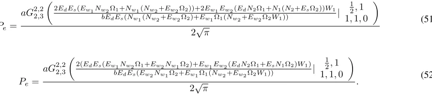
Fig. 6 compares BERs with optimal allocation between the case when h1 is estimated but with perfect knowledge of h2
and the case when both h1 and h2 are estimated in DCE. d1 = 1, d2 = 1, N1 = 1, N2 = 1, Nw1 = 1, P1 = P2 are assumed and 4-PAM modulation is examined. P2 can be
used all by data at the relay when the channel has perfect knowledge ofh2whileNw2 = 1,10,20,30are assumed when
h2are estimated, whereP2 has to be shared by data and pilot
by using our optimal power allocation in this case. As can be seen in Fig. 6, asP1/H1(the power per symbol at the source)
increases, all the BERs decrease. This is because with the total power increasing, the BER performance improves. One can also see that BERs with perfect knowledge ofh2give the best
performance and that when Nw2 (the noise power in pilot) increases, the BERs increase. This is because the increase of noise powers deteriorate the BER performances.
0 5 10 15 20 25 30
10−3
10−2 10−1 100
P1/H1, (dB)
B
E
R Perfect knowledge of h2
Nw 2
=1 Nw
2
=10 Nw
2
=20 Nw
2
[image:11.612.360.512.181.295.2]=30
Fig. 6. Comparison of BERs with optimal allocation between the case when
h1is estimated but with perfect knowledge ofh2and the case when bothh1
andh2are estimated in DCE.
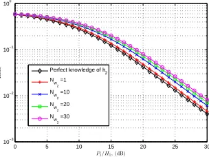
In Fig. 7 and Fig. 8, we compare the BER using the optimal power allocation between Pd, Ps, Pw1, Pw2 under fixedPT with the BER using equal power allocation without
optimization where Pd = PTHD, Ps = PTHD, Pw1 =
PT W1
H
and Pw2 =
PT W2
H . We set d2 = 1 and N1 = 1 in Fig. 7
and Fig. 8. 4-PAM modulation is used as examples and other modulation can be checked in a similar way.
Fig. 7 shows the BERs vs.PT/H when bothh1andh2are
estimated in DCE. Fig. 8 shows the BERs vs. PT/H when
Gdf ix2 and Gwf ix2 are used in CCE. d1 is decreased from 1/4 d2 in Fig. 7 (a) and Fig. 8 (a) to 1/10 d2 in Fig. 7 (b)
and Fig. 8 (b), respectively. From Fig. 7 and Fig. 8, one can see that the BERs with optimal power allocation outperform the BERs with equal allocation under the same conditions. Comparing the system with Nw2 =Nw1 =N2=N1 in Fig. 7 (a) and Fig. 7 (b), one can see that the BER improves when
d1 (the distance between source and relay) decreases. This
is because when d1 decreases, the average power increases
and thus, the BER performance improves. Also, in this case, as d1 is decreased from 1/4 d2 in Fig. 7 (a) to 1/10 d2 in
Fig. 7 (b), the performance gain of optimal allocation over equal allocation is increased from 2 dB to 3 dB. This is because equal allocation can not perform well when the status of source-to-relay channel is different from that of the relay-to-destination channel. Therefore, with the decrease ofd1, the
difference between d1 and d2 becomes larger such that the
performance gain will increase accordingly. As can be seen in Fig. 7 (a), with the increase of Nw2 and N2 from N1 to 3N1, the performance gain increases from 2 dB to 2.25
dB. Also, with the increase of Nw2 and Nw1 from N1 to 3N1, the performance gain increases from 2 dB to 2.4 dB.
[image:11.612.59.292.204.294.2]