On the distribution of the maximum value of the characteristic polynomial of GUE random matrices

warwick.ac.uk/lib-publications

Original citation:

Fyodorov, Y. V. and Simm, Nick. (2016) On the distribution of the maximum value of the characteristic polynomial of GUE random matrices. Nonlinearity, 29 (9). pp. 2837-2855.

Permanent WRAP URL:

http://wrap.warwick.ac.uk/81896

Copyright and reuse:

The Warwick Research Archive Portal (WRAP) makes this work of researchers of the University of Warwick available open access under the following conditions.

This article is made available under the Creative Commons Attribution 3.0 (CC BY 3.0) license and may be reused according to the conditions of the license. For more details see:

http://creativecommons.org/licenses/by/3.0/

A note on versions:

The version presented in WRAP is the published version, or, version of record, and may be cited as it appears here.

Nonlinearity

On the distribution of the maximum value

of the characteristic polynomial of GUE

random matrices

Y V Fyodorov1 _{and N J Simm}2

1 _{Queen Mary University of London, School of Mathematical Sciences, London E1}

4NS, UK

2 _{University of Warwick, Mathematics Institute, Gibbet Hill Rd, Coventry CV4 7AL, UK}

E-mail: [email protected] and [email protected]

Received 28 May 2015, revised 27 May 2016 Accepted for publication 20 July 2016 Published 10 August 2016

Recommended by Professor Alexander R Its

Abstract

Motivated by recently discovered relations between logarithmically correlated Gaussian processes and characteristic polynomials of large random N×N matrices H from the Gaussian unitary ensemble (GUE), we consider the problem of characterising the distribution of the global maximum of D xN( ): log det= | (xI−H)| as N→∞ and x∈ −( 1, 1). We arrive at an explicit expression for the asymptotic probability density of the (appropriately shifted) maximum by combining the rigorous Fisher–Hartwig asymptotics due to Krasovsky [34] with the heuristic freezing transition scenario for logarithmically correlated processes. Although the general idea behind the method is the same as for the earlier considered case of the circular unitary ensemble, the present GUE case poses new challenges. In particular we show how the conjectured self-duality in the freezing scenario plays the crucial role in our selection of the form of the maximum distribution. Finally, we demonstrate a good agreement of the found probability density with the results of direct numerical simulations of the maxima of DN (x).

Keywords: random matrix, log correlated, extreme value, characteristic polynomial, Gaussian free field, GUE, multiplicative chaos

Mathematics Subject Classification numbers: 15B52, 60B20, 60G70, 60G15, 60G57

(Some figures may appear in colour only in the online journal) Y V Fyodorov and N J Simm

On the distribution of the maximum value of the characteristic polynomial of GUE random matrices

Printed in the UK 2837

NON

© 2016 IOP Publishing Ltd & London Mathematical Society 2016

29 Nonlinearity

NON

0951-7715

10.1088/0951-7715/29/9/2837

Paper

9 2837

2855 Nonlinearity

London Mathematical Society

Original content from this work may be used under the terms of the Creative Commons Attribution 3.0 licence. Any further distribution of this work must maintain attribution to the author(s) and the title of the work, journal citation and DOI.

1. Introduction

The space of all N×N Hermitian matrices H with probability density function

P H_{( )∝}exp 2 Tr₍₋ N _{( ))}H2

(1.1) is known as the Gaussian unitary ensemble (or GUE) [1, 36, 41]. Here and henceforth the variance is chosen to ensure that asymptotically for N_→∞, the limiting mean density of the GUE eigenvalues is given by the Wigner semicircle law _{ρ( ) ( / )}x ₌ 2_π 1₋x2 _{supported in the}

interval x∈ −_[ 1, 1_]. The characteristic polynomial p x_{N( )}=det₍xI−H₎ of the matrix H con-stitutes one of the most basic quantities of interest, encoding all eigenvalues of H through the roots of pN(x). As one varies the argument x over an interval containing many eigenvalues for

a given realization of the ensemble, the value of the polynomial pN(x) shows huge variations

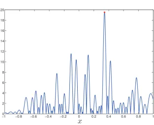
by the orders of magnitude for large N, see figure 1 for N = 50 and figure 2 for N = 3000. The purpose of this article is to describe the statistical properties of the highest peak dis-played by the modulus of the GUE polynomial |p x_{N( )}|, namely the probability density for the maximum value attained by |p x_{N( )}| over the interval [−1, 1] on the real line as N_→∞. Our main result is the following

Conjecture 1.1. Consider the random variable E

{ ( ) ( ( ) )}

[ ]

= | | − | |

∗

∈ −

MN: max 2 log p x 2 log p x .

x 1,1 N N

(1.2)

Then in the limit N→∞ we have

M 2 logN 3 N o y o

2log log 1 1 1

N= ( )− ( ( )) (− + ( )) + ( )

∗

(1.3)

where y is a continuous random variable characterized by the two-sided Laplace transform of its probability density:

CK

s s G s

G s G s

e 1 1 3 7 2

6 1

ys s 2

( ) ( ) ( ) ( / )

( ) ( )

E = Γ + Γ + +

+ +

(1.4)

where Γ_{( )}z and G(z) stand for the Euler gamma-function and the Barnes digamma-function, correspondingly. The value of the constant K is predicted to be K = 4. The normalization C can be evaluated explicitly as

C

A

e 2

1 4 5 2 9 11 12 3

/ / / π

= ₊

(1.5)

where A is the Glaisher–Kinkelin constant A₌e1 12/ − −ζ′( )1 ₌1.282 427 1291..._.

Remark 1.2. The product form of the Laplace transform (1.4) offers an interesting inter-pretation of the above results. Noting that Γ +(1 s) is the moment generating function of a standard Gumbel random variable G, we can write

y=G+ ′y

(1.6)

where y′ is an independent random variable with two-sided Laplace transform

CK

s G s

G s G s

e 1 3 7 2

6 1 .

y s s 2

( ) ( ) ( / )

( ) ( )

E = Γ + +

+ +

′

That (1.7) is indeed the Laplace transform of a bone-fide random variable y′ may be inferred from the work of Ostrovsky [38, 39]. Indeed, it is straightforward to deduce from theorem 2.4 (see equation (3.5)) of [39] that we can represent y′ as

y′=logK+ +Y logβ2,2( )b

(1.8) Figure 1. A plot of a single realization of |p xN( )|e−Elog|p xN( )| for N = 50. The global

[image:4.595.155.469.82.337.2]

maximum is marked with a red circle.

[image:4.595.157.471.386.583.2]

where β2,2( )b is the so-called Barnes beta random variable with parameters b0=1,b1=b2=5 2/

and Y is an independent random variable with p.d.f. p y 1e ey

2 3 e

y

( )= − _{on R.}

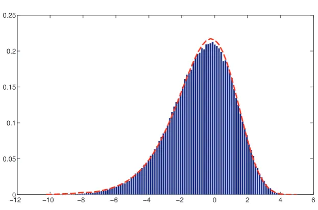
This immediately implies that the probability density of y is the convolution of a Gumbel random variable with y′. Such a convolution structure is expected to appear universally when studying the extreme value statistics of logarithmically correlated Gaussian fields, see the dis-cussion around and after equation (1.12). The distribution of y′ may be obtained numerically by inverting (1.7), as depicted in figure 5.

Remark 1.3. The constant K, which only affects the mean value of y, is conjectured to take the value K = 4 according to our calculations, but numerics (see section 3) seem to suggest a somewhat larger value of K≈2π, and we are less certain that our method allows to reliably predict this constant shift in the mean, see the discussion below (2.27).

In recent years, much interest has accumulated regarding the statistical behaviour of char-acteristic polynomials of various random matrices as a function of the spectral variable x. To a large extent this interest was stimulated by the established paradigm that many statistical properties of the Riemann zeta function along the critical line, that is ζ( /1 2+it), can be under-stood by comparison with analogous properties of the characteristic polynomials of random matrices [2, 11, 13, 29, 30, 32].

For invariant ensembles [36, 41] of self-adjoint matrices with real eigenvalues, statistical characteristics of pN(x) depend very essentially on the choice of scale spanned by the real

vari-able x. From that end it is conventional to say that x spans the local (or microscopic) scale if one considers intervals containing in the limit N→∞ typically only a finite number of eigen-values (the corresponding scale for GUE in (1.1) is of the order of 1/N). At such scales, stand-ard objects of interest are correlation functions containing products and ratios of characteristic polynomials, which show determinantal/Pfaffian structures [5, 6, 7, 28, 33, 43] for Hermitian/ real symmetric matrices and tend to universal limits at the local scale. Similar structures arise for properly defined characteristic polynomials p_{N( )θ =}det₍I₋Ue−iθ_{) of circular ensembles}

(like CUE, COE, and CSE) [36] of unitary random matrices U uniformly distributed with respect to the Haar measure on U(N) (and other classical groups) [8, 11, 12], whose properties on the local scale are indistinguishable from their Hermitian counterparts.

Next, when x spans an interval containing in the limit N_→∞ typically of order of N eigen-values one speaks of the global (or macroscopic) scale behaviour. At such a scale properties of pN (x) display both universal and non-universal features, the latter depending on the ensemble

chosen. The study of characteristic polynomials at such a scale was initiated in [30] where it was shown that the function VN( )θ = −2 log det 1| ( −Ue−iθ)|, with U belonging to the CUE, converges (in an appropriate sense) to a random Gaussian Fourier series of the form

V

n v v

1

e e ,

n

n n n n

1

i i

∑

θ = θ+ θ

= ∞

−

( ) ( )

(1.9)

where the coefficients v vn, n are independent standard complex Gaussian random variables, i.e.

vn 0

{ }

E = , E{ }v2n =0 and E{v vn n}=1. The covariance structure associated with such a pro-cess is given by E{ ( ) ( )}V θ1V θ2 = −2 log e| iθ1−eiθ2| as long as θ1≠θ2. Such a (generalized)

random function V_{( )}θ is a representative of random processes known in the literature under the name of 1/ f noises, see [22, 27] for background discussion and further references.

analogous to that of (1.9), though different in detail. Namely, it was shown that the natural limit of D x˜ ( )N := −log|p xN( )| +E{log|p xN( ) }| is given by the random Chebyshev–Fourier series

F x

n a T x x

1

, 1, 1 ,

n

n n

1

( )=

∑

( ) ∈ −( )

= ∞

(1.10)

with T xn( )=cos arccos(n ( ))x being Chebyshev polynomials and real an being independent

standard Gaussians. A quick computation shows that the covariance structure associated with the generalized process F(x) is given by an integral operator with kernel

F x F y

nT x T y x y

1 1

2log 2 ,

n

n n

1

{ ( ) ( )} ( ) ( ) ( )

E =

∑

= − | − |

= ∞

(1.11)

as long as x≠y. Such a limiting process F(x) is an example of an aperiodic 1/f-noise. Finally, one can consider an intermediate, or mesoscopic spectral scales, with intervals typ-ically containing in the limit N_→∞ the number of eigenvalues growing with N, but represent-ing still a vanishrepresent-ingly small fraction of the total number N of all eigenvalues. The properties of the characteristic polynomials at such scales were again addressed in [23] where it was shown that for the GUE, that object gives rise to a particular (singular) instance of the so-called frac-tional Brownian motion (fBm) [15, 35] with the Hurst index H = 0, again characterized by correlations logarithmic in the spectral parameter.

The discussion above serves, in particular, the purpose of pointing to an intimate con-nection between Gaussian random processes with logarithmic correlations and the modu-lus of characteristic polynomials at global and mesoscopic scales. The relation is important as logarithmically correlated Gaussian (LCG) random processes and fields attract growing attention in mathematical physics and probability and play an important role in problems of quant um gravity, turbulence, and financial mathematics, see e.g. [17]. In particular, the peri-odic 1/f noise (1.9) emerged in constructions of conformally invariant planar random curves [4]. Among other things, the statistics of the global maximum of LCG fields attracted consid-erable attention, see [14] and references therein. Particularly relevant in the present context are the results of Ding, Roy and Zeitouni [14] on the maxima of regularized lattice versions of LCG fields which we discuss informally below. Let VN=ZNd be the d-dimensional box of side length N with the left bottom corner located at the origin. A suitably normalized version of the logarithmically correlated Gaussian field is a collection of Gaussian variables φ_{N v}, :v V∈ N with variance E{φ2_{N v,}}=2 logN+f v( ) and covariance structure

N

u v g u v u v V

, 2 log , , for

N v, N u, N

{ } ( )

E φ φ =

| − | + ≠ ∈

+

(1.12)

where log₊( )w =max log , 0( w ) and both f (v) and g(u, v) are continuous bounded functions far enough from the boundary of VN. Now set MN=maxv V∈ NφN v, and

mN= dlogN−₂3_dlog logN. The limiting law of MN−mN is then expected, after an appro-priate shift and rescaling, to be given by the Gumbel distribution with random shift:

P y lim Prob M m y e ,

N N N

ed y z

{

}

( ) ( ⩾ )

→

( ) E

= − =

∞

− −

(1.13)

random variable Z₌e− d z _{is related to the so called derivative martingale associated with the} LCG fields [14] whose distribution is however not known. Recently it has been shown that the recentering term mN in (1.13) also holds for a randomized model of the Riemann zeta

func-tion [2], proved by revealing a special branching structure within the associated logarithmic correlations.

We see that our conjecture 1.1 for the maximum of characteristic polynomial of large GUE matrices fully agrees with the predicted structure of the maximum of LCG in dimen-sion d = 1. Note that the expresdimen-sion (1.13) implies that the double-sided Laplace transform of

the density y P y

y

d d

( ) ( )

ρ = − for the (shifted) maximum y is related to the density ρ_{˜( )}z of the random variable z as

y y s z z s

eys e dsy 1 e dsz 1 ezs

( ) ( ) ( ) ˜( ) ( ) ( )

E =

_∫

ρ = Γ +

_∫

ρ = Γ + E

(1.14)

which is in turn equivalent to the Gumbel convolution in equation (1.6). In fact our formula (1.7) provides the explicit form of the distribution for the derivative martingale of our model, thus going considerably beyond the considerations of [14].

From a quite different perspective, processes similar to (1.9) and (1.10) appeared in the context of statistical mechanics of disordered systems when studying extreme values of ran-dom multifractal landscapes supporting spinglass-like thermodynamics [3, 20, 25, 27]. The latter link is especially important in the context of the present paper. The idea that it is ben-eficial to look at |p_{N( )}θ | as a disordered landscape consisting of many peaks and dips, and to think of an associated statistical mechanics problem was put forward in [21, 22]. It allowed to get quite non-trivial analytical insights into statistics of the maximal value of the CUE polynomial sampled over the full circle θ∈[0, 2π] , or over its mesoscopic sub-intervals. This was further used to conjecture the associated properties of the modulus of the Riemann zeta-function along the critical line, see some recent advances inpired by that line of research in [2]. Some relations between between CUE characteristic polynomials and logarithmically correlated processes (in the form of the so-called ‘multiplicative chaos’ measures introduced by Kahane, see [42] for a review) was recently rigorously verified in [46]. The case of GUE polynomials however remained outstanding. We point out in a subsequent paper, the position x* _{where the maximum value M}

N

∗ _{is attained was studied in [24].}

It is our objective in this paper to provide two separate means of supporting conjecture

1.1. First, we will provide careful and explicit, albeit in part heuristic, analytical argu-ments. Although our technique is inspired by the approach of [22] it contains new non-trivial features necessary to overcome challenges arising from the non-uniform eigenvalue density ρ_{( )}x, reflecting absence of translational invariance for the GUE at the global spec-tral scale (note e.g. the non-trivial recentering in (1.2)). All this makes actual calculation for the GUE much more involved in comparison to the CUE and the limiting random vari-able u above appears to be more complicated than its CUE counterpart. Secondly, we will test our conjecture with numerical experiments for matrices of size N = 3000 and around 250 000 realizations. This is especially important as part of our analysis is based on very plausible but as yet not fully rigorous considerations. Finally, is natural to expect that the same distribution should be shared by the maximum modulus of characteristic polynomials for Hermitian random matrices with independent entries taken from the so-called Wigner ensembles, see [18].

p x C 1 x N 2 e j

k N j

j k

j j x N

1

2

1

2 2 2 1 2 log 2

j 2j 2j 2j j

( ) ( )( ) ( / )/ ( ( ))

E⎛

⎝

⎜⎜

∏

| |α⎞_⎠⎟⎟=

∏

α − α α α

= =

− −

(1.15)

x x O N

N

2 1 log

i j k

i j

1

2 i j

( )

⩽ ⩽

⎜ ⎟

⎡

⎣⎢ ⎛⎝ ⎞⎠ ⎤ ⎦⎥

∏

× | − | α α +

<

−

(1.16)

where

C G

G

: 2 1

2 1

2 2 2

( )α ₍(α )₎

α

= +

+

α

(1.17)

and G(z) is the Barnes G-function. Differentiating with respect to α, we deduce that

p x N x O N N

2 log _N 2 2 1 2 log 2 log ,

( ( ) ) ( ( )) ( ( )/ )

E | | = − − +

(1.18) where we used that C′( )0 =0.

The most salient feature of the asymptotics (1.16) is the product of differences on the sec-ond line, which when rewritten in the form

x x

exp 2 log 2 ,

i j k

i j i j

1

( )

⩽ ⩽

⎡ ⎣ ⎢ ⎢

⎤ ⎦ ⎥ ⎥

∑

α α

− | − |

<

(1.19)

can be looked at as evidence of the limiting Gaussian process (1.10) with logarithmic cova-riance (1.11) in the background. We will however stress that naively replacing the (shifted)

p x

log| _N( )j | with the corresponding 1/f noise (1.10) is not a valid approximation as the factors

x

1 2_j 2j2

( ₋ )α/ _{in (1.16) do play an essential role in determining the extreme value statistics of}

p x_N( )j

| |. Let us finally note that had we suppressed the factors C( )αj the faithful descrip-tion of log|p x_N( )j | would be that of the regularized LCG process with covariance (1.11), the position-dependent variance 2 logN₊2 log1₂ 1₋x2 _{and the position-dependent mean}

N x₍2 2_{− −}1 2 log 2_{( )).}

2. Statistical mechanics approach to the distribution of GUE characteristic polynomials

Following the ideas of [22] we recast the problem of computing the value of the global maxi-mum of |p x_{N( )}| (with an appropriate shift by the mean value) as a statistical mechanics prob-lem characterized by the partition function

N

x x q

2 e d , 0, 0

N x q

1 1

N

( )_{β =}

_∫

βφ ( )_ρ( ) _β> ⩾

− −

Z (2.1)

with the ‘potential’φ_N( )x = −2 log( |p x_N( )| −Elog|p x_N( ) )|, inverse temperature β>0 and β -independent non-negative parameter q. Specifically, if we define the associated ‘free energy’

as F( )β = −β−1logZN( )β , then

β = φ = − | | − | |

βlim→∞F( ) x∈ −min( 1,1) N( )x 2 max logx∈ −( 1,1)[ p xN( ) Elog p xN( ) ].

(2.2)

when taking the limit β→∞, we will actually see that it plays a very important role in sup-porting our procedure of extracting the free energy for β exceeding some critical value.

Now we aim to compute the integer moments of the partition function defined in (2.1):

⎜ ⎟ ⎛ ⎝ ⎞⎠ ⎛ ⎝ ⎜⎜ ⎞_⎠⎟⎟

∫

∫

∏

∏

β = … | |β β ρ

− − _{= =}

− | |

N

p x x x

2 e d .

N k k j k N j j k

p x q j j 1 1 1 1 1 2 1

2 log N j

Z

E_{( ( ))} E _{( )} E ( ) _{( ) (2.3)}

In the limit N_→∞ the leading asymptotics of the above integral can be extracted by replacing the factor k_j p x

N j

1 2

(

( )

)

E ∏ | |β

= with its asymptotics from (1.16). In this way one obtains

⎜ ⎟ ⎛ ⎝

⎜⎜⎛_⎝ ⎞_⎠ ⎞_⎠⎟⎟

_∫

∏

∏

β ∼ +β β π − β | − | β …

− ₌

+ <

−

N

C x x x x x

2 2 1 2 d d .

N k q k j k j q

i j k

j i k

1 1,1 ₁ 2 ₂ 1 2 1 k 2 ₂ 2 Z

E( ( )) ( )( / ) ( ) ( )

[ ] _{⩽ ⩽}

(2.4) After changing variables xj=2yj−1 the integral above assumes the form

y y y y y y

2k q k k 1 d d

j k j q j q

i j k i j k

1 2 1

0,1 ₁ 2 ₂ 1 2 1 k 2 2 2 ₂ 2 ( ) ( ) ( ) [ ] _{⩽ ⩽}

∫

∏

−

∏

| − | …

β+ + − β − β β β

=

+ ₊

<

− _(2.5)

S q q

2

2 , 2 ,

k q k k

k

1 2 1 2 2 2

2 2

( ) ( ) ⎛

⎝

⎜β β β ⎞_⎠⎟

= β+ + − β − + + −

with the quantity S a bk( , ,−γ) being the well-known Selberg integral [19]:

S a bk , , : x 1 x x x dx dx

j m

j a

j b i j k

i j k

0,1 _{1 1}

2 1 k ( ) ( ) [ ] _{⩽ ⩽}

∫

∏

∏

γ

− = − | − | γ …

= <

−

(2.6)

a j b j j

a b k j

1 1 1 1 1

2 2 1

j k

1

( ( ) ) ( ( ) ) ( )

( ( ) ) ( )

∏

γ _γ γ _γ γ

= Γ + − − Γ + − − Γ −

Γ + + − + − Γ −

=

(2.7)

( γ)˜ ( γ)

=

Γ − S a b −

1

1 , , .

k k

(2.8)

It is easy to see that the found expression for the partition function moments _{E( )}k

β

Z in (2.5) and (2.4) is well-defined for any 0_{< =γ β}2_<1 _{and for an integer k satisfying 1< <k γ}−1_{. To}

understand how to deal with the case k>_β12, we recall that Krasovsky’s asymptotic formula

(1.16) is valid only when all of the differences | − |xi xj remain finite when N→∞, and should be replaced by a different expression when | − | ∼_{x x N}−

i j 1. One can check that the divergence of the integral for k_>1_/β2 _{is due precisely to the fact that these near degeneracies become}

important. Relying on our experience with the corresponding situation for the CUE [22] case suggests that taking into account the correct short-scale cutoff cures the formal divergence, but changes the asymptotics of the moments _{E( )}k

β

Z with N: namely, these become of the order of N1₊k2 2_β

for k_>β−2 _{whereas they are of the order of N(}1_+β2₎k

for k_<β−2_{. Such a change of}

validated by extending the theory of [10] from Toeplitz to Hankel case. Actually, as argued in [20] the moments with k_>β−2 _{play only a secondary role when addressing the question}

of extreme value statistics which is controlled exclusively by moments with 1_{< <}k _β−2_{. Our}

next goal is to use the latter integer moments for restoring the associated part of the probability density P Z( )β for the partition function. This will be achieved if we manage to find the

distri-bution for a random variable z_β whose positive integer moments are given by

γ β γ β

= − = = + =

β

z S a b, , , a b q

2 , .

k k

2

2

E( ) ˜ ( )

(2.9)

Such a task actually requires finding a way to continue analytically those moments to complex k. Below we will arrive at the required continuation by exploiting a relatively simple heuristic procedure suggested in [25]. Note that in a series of insightful papers [37–40] Ostrovsky developed a rigorous mathematical procedure of the required continuation which provides an a posteriori justification of the results obtained via the heuristic approach.

2.1. Analytical continuation of Selberg’s integral

One starts with finding a recursion satisfied by S a b˜ (k , ,γ) for integer k which is suitable for the continuation. By writing

a b k j a b k

a b k

a b k j

a b k

2 3 2 2

2 2 2

2 2

2 2 3

j k

j k

1 1

1

∏

γ γ

γ

γ γ

Γ + + − + − = Γ + + − −

Γ + + − −

∏ Γ + + − + −

Γ + + − −

= −

=

( ( ) ) ( ( ) )

( ( ) )

( ( ) )

( ( ) )

(2.10) one sees immediately that

E E

( )

( )

( ( ) ) ( ( ) ) ( ) ( ( ) )

( ( ) ) ( ( ) )

γ γ γ γ

γ γ

=Γ + − − Γ + − − Γ − Γ + + − −

Γ + + − − Γ + + − −

β

β− z z

a k b k k a b k

a b k a b k

1 1 1 1 1 2 2

2 2 2 2 2 3 .

k

k 1

(2.11) It is convenient to introduce the moments M sβ_{( )} of the random variable zβ defined for any

complex s as M sβ_{( )}=_E(z1β−s₎ . We then have E( )zβk =M(1−k) (,Ezkβ−1)=M(2−k) and

after identifying s = 1 − k the recursion (2.11) takes the form M s

M s

a s b s s a b s

a b s a b s

1

1 1 1 1 2 1

2 2 2 2 1

( )

( ) ( () ( ) () ( ( ) ) (( ) ) ( ) )

γ γ γ γ

γ γ

+ =

Γ + + Γ + + Γ + − Γ + + + +

Γ + + + Γ + + + +

β

β (2.12)

which is now assumed to be valid for any complex s. It is convenient to further use the duplica-tion formula for the Gamma funcduplica-tion:

z z z

2 22z 1 1 2

( ) _π ( ) ( / )

Γ (2.13)= − Γ Γ +

to get rid of the argument 2s in the denominator. Indeed, we have

a b s s a b s a b

a b s

s a b s a b

2 2 2 1 2 3 2

2 2 1

2 1 1 2 2 1 2 3 2

a b s

a b s

1 2

1 2 1

( ) ( ( )/ ) ( ( )/ )/

( ( ))

( ( / ) ( )/ ) ( ( / ) ( )/ )/

( )

γ γ γ π

γ

γ γ π

Γ + + + = Γ + + + Γ + + +

Γ + + + +

= Γ + + + + Γ + + + +

γ

γ

+ + +

+ + + +

( )

( ) ( ( () ( / ) ( ) ()/ ) ( (( )) (/ ) ( ()/ ) ) )

( ( )/ ) (( )/ )

( ) ( )

γ γ γ γ

γ γ

π

γ γ

+ =

Γ + + Γ + + Γ + − Γ + + + +

Γ + + + + Γ + + + +

×

Γ + + + Γ + + +

β β γ + + + + M s M s

a s b s s a b s

s a b s a b

a b s a b s

1

1 1 1 1 2 1

1 1 2 2 1 2 3 2

2

1

1 2 3 2 .

a b s

2 1 4 1 (2.14)

Recalling that according to (2.9) in our particular case a b q

2 2

2

= = +β we now use the param-eterisation a₌a₁₊a_2β2_{, b b b}

1 2β2

= + and β-independent constants a a b b1, , .2 1 2. After this

we finally arrive at M s

M s 1

( )

( + )

β

β

(2.15)

β β β β

β β

π

β β

= Γ + + + Γ + + + Γ + − Γ + + + + + +

Γ + + + + + + Γ + + + + + +

×

Γ + + + + + Γ + + + + +

β

− + + − + + +

a s a b s b s a b s a b

s a b a b s a b a b

a b s a b a b s a b

1 1 1 1 2 1

1 1 2 2 2 2 1 2 3 2

2

1 2 2 3 2 2 .

a b s a b

1 2 2 1 2 2 2 1 1 2 2 2

2

2 2 1 1 2 2 2 1 1

2 1 4 1 2 2

1 1 2 2 2 1 1 2 2 2

1 1 2 2 2

( ( )) ( ( )) ( ( )) ( ( ) )

( ( / / / ) ( )/ ) ( ( ( )/ ) ( )/ )

( ( )/ ( ( )/ )) (( )/ ( ( )/ ))

( ) ( )

(2.16)

To determine the function M s_{β( )} which satisfies (2.16) for any complex s we follow [25] and introduce a variant of the Barnes function G x_{β( )} which for any R( )x >0 is defined by:

⎛ ⎝

⎜⎜ ⎞_⎠⎟⎟

G x x Q t

t Q x

Q x

t

log 2

2 log 2

d e e

1 e 1 e

e 2 2 2 t xt t t t 0 2 Q 2

∫

π = − + − − − + − + −

β _{β β}

∞ − − − − − ( ) / ( ) ( )( ) ( / ) / / (2.17) where Q= +β 1/β. This function satisfies the so-called self-duality relation

G xβ( )=G1/β( )x

(2.18) and further posesses a shift property that is central for our studies

β β π β

+ = Γ

β β

β

β

− −

G x_{( )} 1 2/ x_{( )}2 ₂1 _{( ) ( )}x G x .

(2.19)

One can check that G xβ_{( )} for β=1 coincides with the standard Barnes function G(x) which

is a unique solution of the recursion G x( +1)= Γ( ) ( )x G x satisfying G(1) = 1. Similarly to the standard Barnes function the general Barnes G xβ_{( )} has no poles and only zeroes located

at x= −nβ−m_/β, n, m = 0, 1, ... A detailed discussion of properties of functions closely related to G xβ_{( )} can be found in [38, 39], see the appendix and lemma 1 for more details.

Let us now define a function M( )G_{( )}s

β of the complex argument s by

π β β β β β β β β β = × + + + + + + + + × + + + + + + + + − + β β

β _β β _β

β _β β _β

β _β β _β

β _β β _β

− + + + + + + + + + + + + + + + + + + +

(

) (

)

(

) (

)

(

) (

)

(

) (

)

(

)

(

)

(

)

(

)

( ) ( ) ( ) ( ) ( ) ( ) M s

G s G s

G s a G s b

G s G s

G s a b G s

2

1 1

G s B s B s s

a b a b a b a b

a b

a b a b a b a b

a b 1 2 2 2 2 2 2

2 1 2 1

1 2 3 2 2 3 2

2 2 2 1

12 2 2

2 2 1 1 2 2 1 1

1 1

2 2 1 1 2 2 1 1

1 1

(2.20)

where B1=2β2 and B2=2(a1+b1+1)+β2(2a2+2b2−1). Then a straightforward

G s c

G s c c s

1

2 ₂1 1 2 2s c 2

( ( ) / )

( / ) ( ) / ( )

β β

β β π β β

+ +

+ = Γ +

β

β

β− _{−β −}

(2.21)

shows that the ratio _MMGG_ss₁

( ) ( ) ( ) ( ) ₊

β

β reproduces the right-hand side of (2.16) from which we conclude

M s

M s

M s M s

1 1

G

G

( )

( )

( )

( )

( )

( ) ₊ = ₊

β

β

β

β

(2.22)

which finally implies that

M s M s M

M

1 1 G

G

( ) ( ) ( )

( )

( ) ( ) =

β β β

β

(2.23)

where Mβ( )1 ≡1. Together with (2.4) and (2.5) and the fact that Mβ( )1 =1, we obtain for

1 β< :

⎛

⎝ ⎜ ⎜ ⎜

⎞

⎠ ⎟ ⎟ ⎟

β β π

β ∼

Γ −

β

β β β

β −

+ −

− + + + −

C M s

M

2

1 2 1 .

N s

N q s

s q s s

G

G

1 2

1

2 1

1 1 2 1

2

2 2

Z

E( ( ) )

( )

₍ ( )( / )₎ ( )

( )

( )( ) ( ) ( )

( )

(2.24)

2.2. Duality and the freezing transition

The pair (2.20)–(2.23) solves the problem of finding the complex moments M sβ_{( )}=_E(z1β−s₎

of the random variable zβ for any complex s, and β<1. Knowledge of such moments can be

used to restore the probability distribution of zβ, hence of the partition function ZN( )β , and of its logarithm (the free energy) for large N1. Our goal is however to study the limit of the latter as β→∞ and one therefore should have a way of extracting information on the distri-bution for β>1. In doing this we rely on the freezing transition scenario for logarithmically correlated random landscapes. The background idea of such scenario goes back to [9] and was further advanced and clarified in the series of works [20, 25–27]. In brief, this scenario predicts a phase transition at the critical value β=1 and amounts to the following principle:

Thermodynamic quantities which for β<1 are self-dual functions of the inverse temperature β, i.e. functions that remain invariant under the transformation_β→β−1_,

retain for allβ>1 the value they acquired at the point of self-duality β=1.

Although such a scenario is not yet proven mathematically in full generality and has the status of a conjecture supported by physical arguments and available numerics, recently a few nontrivial aspects of freezing were verified within rigorous probabilistic analysis, see e.g. [3,

14, 44] for efforts in this direction.

Within that scenario, one of the main outcomes of the analysis performed in [25] is that the self-dual object associated with the distribution of the partition function for logarithmically correlated landscapes is expected to be the appropriately defined Laplace transform:

g y exp e y ,

N eN

( )=E( [− ( )/ ( )] )β β

β βZ Z

(2.25)

N G G

1

2 1 1

4 _. Ne q 1 2 2 2 ( ) [ ( )] ( ) ( ) ( ) _⎜⎛ _⎟ ⎝ ⎞⎠ β β

β β π

= +

+ Γ −

β +

Z (2.26)

Moreover, defining the probability density p y_{β( )} by p y_{β( )}= − ′g y_{β( )} one can show that the double-sided Laplace transform for such a probability density is related to the complex

moments M s

s 1 N N e ˜ ( ) ( ) ( ) ( ) E⎜⎛ ⎟

⎝ ⎞⎠

=

β β_β

− Z

Z of the scaled partition function via the following relation (see equation (26) of [25])

( ) ˜ ⎛_⎝⎜ ⎞_⎠⎟ ⎛_⎝⎜ ⎞_⎠⎟

∫

_β = β +_β + Γ + _β

−∞ ∞

p y y M s s

log e dys log 1 log 1 .

(2.27)

Actually, as shown in [25] the freezing scenario implies that the variable y whose probability density is given by p_{β=1( )}y is precisely the fluctuating part of the height of the global mini-mum of the random potential which is our main object of interest. Note however that the scale

Ne( ) ( )_β

Z diverges when approaching the critical point β=1, and that the associated free energy log _Ne

1 ( )_{( )β}

−_β Z is self-dual only in the leading order, given by _{− +(β β}−1₎logN_{. The latter} term after freezing at β=1 yields the leading 2 logN term in our conjecture equation (1.3) for the maximum, whereas the logarithmically divergent term ₋1log_{Γ −(}1 _β2₎

β after careful

re-interpretation results in the second term 3log logN

2

− , see [27] for the detailed explanation of that mechanism. The procedure leaves however a certain arbitrariness in the terms of the order of unity in the mean free energy, hence in the overall shift of the position of the maximum. Let us stress however that apart from such a shift, the shape of the distribution function recovered in the framework of the freezing paradigm is completely fixed by the procedure.

Our strategy therefore will be to check if self-duality holds for the right-hand side combina-tion in (2.27) when we substitute our expression for the moments. Before we proceed, it will be helpful to further expand our expression (2.24). Inserting (2.20) and making use of the identity

G s s G s 1 1 1 1 1 1 2 s 2

1 2 1 2 2 1

( (β ) / )β ( ( ( / )))( )( )/ / ( )

β

β β π β

− + =

Γ + −

+

β β

β− − −β −

(2.28)

shows that (taking into account all prefactors coming from (2.4), (2.5) and (2.20))

β β π β π β

β β β

β β

β β

β β

∼

× Γ + − + + + +

+ + + +

× + + + +

+ + + + +

β β β β

β

β _β β _β

β _β β _β

β _β β _β

β _β β _β

− − + − − − − − + + + + + + + + + + + + + + + + + + M s

G s G s

G s a G s b

G s G s

G s a b G s

2 2

1

1 1

1 .

N s Ne s B s s s

s

G

a b a b a b a b

a b

a b a b a b a b

a b

1 1 2 1 2 1 2 1

2 1 2 2 2 2 2 2

2 1 2 1

1 2 3 2 2 3 2

2 2 2 1

2

2 2

2

2 2 1 1 2 2 1 1

1 1

2 2 1 1 2 2 1 1

1 1 Z Z E

(

) (

)

(

) (

)

(

) (

)

(

) ( )

(

)

(

)

(

)

(

)

( ( ) ) [ ( )] ( ) ( ) ( ( )) ( ) ( ) ( ) ( ) ( )/ / ( ) ( ) (2.29)

A direct inspection makes it clear that the self-duality is only possible if either a1=a b2, 1=b2

or a1=b b2, 1=a2. For the GUE characteristic polynomials, we have a1=b1=1 2/ ,

from its Laplace transform via (2.27) as the probability density for the (shifted) global mini-mum. Using (2.29) with a1=a2=b1=b2=1₂ we get

s

G s

G s

G s G s

G s G s

c

2

1 1 1

1 2

1

2

N s Ne s s

1 1 1 1

2

3 2

3 2

2 1

2 2

3 1

2

β β

β β

β

β β

β β

∼

× Γ + − + +

+ +

+ + + +

+ + +

β

β _β

β _β

β _β β _β

β _β β _β

β

− − + −

Z Z

E

(

)

(

)

(

(

) (

) ( )

( )

)

( ( )) [ ( )]

( ( )) ( )

( / )

( )

( )

( ) ( )( )

(2.30)

where cβ is a constant determined by the condition E( ( ) )ZN β1−s |s=1=1. Inserting (2.30) into

the right-hand side of (2.27) (which is now manifestly self-dual) leads to the following expres-sion at β=1:

p y y K s M s

CK s

G s G s G s

G s G s G s

CK

s G s s

G s G s

e d 1 1

1 ₁ 7 2 3 4

3 6 2

1 1 7 2 3

1 6 .

ys s

s

s

1 1

2 2

2 2

( ) ( ) ˜ ( )

( ) (₍ / ) (_{) ( ) (}) ( ₎)

( ) ( / ) ( )

( ) ( )

∫

= Γ + +

= Γ + + + +

+ + +

= Γ + + Γ +

+ +

β β

−∞ ∞

= =

(2.31)

where C=cβ=1 and K = 4 is a constant which determines the shift in the maximum as

dis-cussed below (2.27). The latter formula (2.31) constitutes our main analytical result and finally leads to our conjecture 1.1.

3. Numerical study of the distribution of the maximum modulus of GUE characteristic polynomials

The purpose of this section is to provide a numerical test of conjecture 1.1, but for the reasons described below (2.27) there is some freedom in our choice of the shift K, for which numer-ically K=2π seems to give the best fit, and is what we test against below. We emphasize that the value of K only shifts the mean value of the distribution, all other aspects of the distribution being fixed uniquely by the freezing scenario.

3.1. Results

In figure 3 we present a histogram of the recentered and rescaled maximum of the GUE char-acteristic polynomial, defined by

y∗_N:=₍2 log_{( ) ( / )}N − 3 2 log log_{( ( ))}N −M∗_N+c∗_N)(1+s∗_N)

(3.1)

s y M

c y s N N M

Var Var 1

1 2 log 3 2 log log ,

N N

N N N

( )/ ( )

( )/( ) ( ( ) ( / ) ( ( )) )

E

= −

= + − − −

∗ ∗

∗ ∗ ∗

(3.2)

as derived by requiring _{E( )}y∗_N =_{E( )}y _{and Var y Var y}

N

( )∗ = ( )_{. In table 1 and figure 4 we display}

values of the parameters c_N∗ and s_N∗ for the studied range of sizes N, as determined empirically from the mean and variance of the random variable u. The observed decay with N is cer-tainly consistent with asymptotic validity of our conjecture 1.1, though the convergence to the asymptotic results is too slow to make more definite claims. To resolve further decrease of the coefficients c∗_N and s∗_N would require much larger matrices and is computationally demanding.

Finally, we provide a numerical validation of the decomposition (1.6). In figure 5 we plot the inverse Laplace transform of (1.7) obtained by a direct numerical evaluation of the integral in the Bromwich inversion formula for the Laplace transform. The positive and normalized curve clearly corresponds to a bona fide probability density of some real random variable y′.

3.2. Numerical method

The numerical evaluation of the maximum value (1.2) may be considered quite a non-trivial problem in its own right, for at least two reasons. Firstly, the characteristic polynomial pN (x)

Figure 3. The centered and scaled maximum as defined by (3.1). The dashed line is the probability density of the random variable y given in Laplace space by (1.4).

Table 1. Finite-N corrections for increasing values of N all with 250 000 realizations.

N c∗N s∗N

[image:15.595.153.465.87.293.2]

having zeros as the eigenvalues of H, displays O(N ) oscillations in the spectral interval [−1, 1] with hugely varying peaks heights. This produces considerable clusterings of ‘near-maxima’

[image:16.595.99.467.86.327.2]

which may confuse any naive attempt to find the true maximum value. Secondly, the slow changing nature of the correction terms in conjecture 1.1, of order log( )N and log log( )N ) respectively, require one to go to somewhat large matrices to resolve reasonable asymptotic behaviour. The problem is further compounded by the numerical instability of calculating determinants of such matrices.

Figure 4. Each triangle represents a value of c∗N obtained from (3.2) with 250 000

realizations.

[image:16.595.155.464.368.565.2]

Our solution to these problems heavily relies on a sparse realization of GUE matrices H originally due to Trotter [45] (see also Dumitriu and Edelman [16]). He discovered that the eigenvalues of GUE matrices H have the same joint probability density as those of the follow-ing real symmetric tri-diagonal matrix:

N

1 2 2

0, 2

0, 2

0, 2

0, 2

N N

N

2

2 4

2 2 2 1

2 1

( )

( )

( )

( )

( ) ( )

( )

⎛

⎝ ⎜ ⎜ ⎜ ⎜ ⎜ ⎜

⎞

⎠ ⎟ ⎟ ⎟ ⎟ ⎟ ⎟

χ

χ χ

χ χ

χ =

− −

−

H

N

N

N

N

(3.3)

where N( )0, 2 is a normal random variable with mean 0 and variance 2. The sub-diago-nal is composed of random variables χ2_n having the same density as χ22n where χ22n is a

χ-square random variable with 2n degrees of freedom. To compute the maximum value of p x_N( )=det(xI−H)=det(xI−H), we begin by exploiting the known asymptotic behaviour

p x N x o

2 log_{E | N( )|= (}2 2_{− −}1 2 log 2_{( ))+ ( )}1

(3.4) so that

= | |− | | ∼ | − − − − |

f x_N : 2 log p x_N 2 log p x_N 2 log det e x2 1 2 log 2 xI .

H

E

( ) ( ) ( ) ( ( / ( ))( )) _(3.5)

Further progress is now possible thanks to the fact that determinants of tri-diagonal matrices satisfy a linear recurrence relation. Furthermore, by an appropriate rescaling, the recursion computes determinants of all leading principal minors simultaneously, thus computing fj (x)

for all j= …1, ,N in linear time.

Now to find the maximum, we define a mesh M= − + ∆_{ 1 n_/ :n= … ∆0, , 2 _} with N

2

∆ ∼ and evaluate fN (x) at each of the points in M. At those points where fN (x) is maximal

the Matlab function ‘fminbnd’ is invoked to converge onto the global maximum. Figure 2

illustrates the complexity of the problem. Our algorithm is sufficiently precise to distinguish the true maximum (located at x≈ −0.3 in red) from other possible candidates, e.g. x≈ −0.7 as well as the thousands of other local maxima.

Acknowledgments

We are grateful for helpful comments from Christian Webb during the preparation of this manuscript. We would like to thank Dmitry Ostrovsky and Pierre Le Doussal for enlightening discussions and suggestions. In particular, we thank Dmitry Ostrovsky for pointing out the connection between (1.7) and the Barnes Beta distributions of [39]. We acknowledge support from EPSRC grant EP/J002763/1 ‘Insights into Disordered Landscapes via Random Matrix Theory and Statistical Mechanics’.

Appendix. Equivalence between analytic continuations of the moments and connection to the Alexeiewsky–Barnes G function

In a more recent arXiv submission [24], a different analytic continuation to M( )G_{( )}s

β in (2.20) is

given for the moments of the partition function. Indeed, denoting M( )_βG( )s =_E(z1β−s) as before

M s C G s a b

G s G s a G s b G s a b

2 G

a b, ,

2

1 1 1 2

( ) ˜ ( )

˜ ( ) ˜ ( ) ˜ ( ) ˜ ( )

( ) β

β β β β β β

= + + +

+ − + + + + + + + +

β β

β _β

β _β β _β β _β β _β

(A.1) where a =_β1a1+βa2, b =_β1b1+βb2,

G x : G x 2 2x 2 x Q 22 x ₂1 1₂

˜ ( )_{β β = β}( )_{β β}β / −β β( )/ ( )_π β( _β− )

(A.2)

and C_{a b, ,β} is a normalizing constant ensuring M( )G_{( )}1 ₌1

β . The purpose of this appendix is to

show that the resulting formulae are equivalent: that M( )G_{( )}s ₌M( )G_{( )}s

β β . Our method is based

on the ideas of [38], in particular the properties of a function there denoted G x_{( )}|τ and known as the Alexeiewsky–Barnes G function, see [38] equations (8)–(11). First we need a lemma, which is stated without proof in the bibliography of [24].

Lemma A.1. For any Re( )x >0 and Re( )β >0, we have

˜ ( )

˜ ( ) ( )

β

β = |β

β

β

−

G x

G G x .

2

(A.3)

Proof. We start with the integral representation, formula (84) in [38], that for Re( )x , Re( )τ >0, we have ( ) ( ) ( ) ( )( ) ( ) ⎡ ⎣⎢ ⎤ ⎦⎥

∫

τ τ | = − − + − + − + − − − τ τ τ τ ∞ − − − − −

G x t

t

x

x x x

log d 1

e 1 1 e

e 2

1 e

e 1 1 e .

t t

t t x

t t

0

2 1 _(A.4)

Now setting _τ=1_/β2 _{and changing variables t→tβ in (A.4), we insert the integral}

represen-tation (2.17) into E x_{( )}: log₌ G˜ ( )_βx ₋logG x_{( |β} 2₎₋logG˜ ( )_β

β β − β . The latter is a quadratic

polynomial in x: E x_{( )=}a x2₊b x₊c

β β β β. The reason is that after the change of variables, the

terms of the form e−txβ_/((1₋e−βt₎₍1₋e−t/β_{)) completely cancel. Some algebra shows that the}

first two coefficients of the resulting polynomial are

a t

t

2 log 2

d _{e t e t}

2

2 0

( ) /

_∫

[( / )]

β _{β β}

= + − β β ∞ − − (A.5) b t t t 1 2log 2

d 1 e 1 e 2 t t 0

( )π

_∫

⎡_⎣⎢ β _/ / ⎤_⎦⎥

= + − + − − β _β β ∞ − (A.6) ⎡ ⎣⎢ ⎤⎦⎥

∫

π = + − + − +

∞ _t −

t t

1 2log 2

d 1 1

e 1 e 2 . t t 0 ( ) (A.7)

The fact that aβ≡0 is a famous integral known as Frullani’s integral. That the expression (A.7) vanishes can be deduced from the limit τ→0 of identity (A.37) in [38]. Finally, to see that cβ≡0, it is enough to notice that Eβ( )1 ≡0, which follows from the fact that G( )1| ≡τ 1,

equation (9) in [38]. □

Corollary A.1. We have =

β β

M( )G_{( )}s M( )G_{( )}s.

Proof. The proof follows immediately from a doubling formula for G x_{( |β}−2_{) studied in}

[38]. From lemma 1 and equation (77) in [38] it follows that

G 2z C 2 z 21 2z2 z 1

˜ ( )_{β = β}( )_π−/β + −(β+ / )β

(A.9)

β β β β

×G z G z˜ ( ) ˜ (β β + / ) ˜(2 G z+1 2/( )) ˜ (G zβ + /2+1 2/( ))

(A.10)

where C_β is a constant depending only on β. Using this with z s 1 a b

2

β

= + +_β + in (A.1) exactly reproduces all of the correct G_β factors in (2.20). The pre-factors π−s B s2 12+B s2ββ2s fol-low from transforming G˜β to Gβ as in (A.2) and

C

2 z 2 z z 2

a b s s s a b

2 1

, ,

2 2 2 2 2

2 2 2 2

( )_π /β (β / )β ₌ ( ) _π ( )

β β β β β

− − + − + + − +

(A.11)

with constant C( )2_{, ,a b}

β whose final contribution is fixed by the normalizations Mβ( )G( )1 =

=

β ( )

( )

M G 1 1_{. □}

References

[1] Anderson G W, Guionnet A and Zeitouni O 2009 An Introduction to Random Matrices (Cambridge: Cambridge University Press)

[2] Arguin L-P, Belius D and Harper A J 2016 Maxima of a randomized Riemann zeta function, and branching random walks Ann. Appl. Probab. at press

[3] Arguin  L-P and Zindy  O 2014 Poisson–Dirichlet statistics for the extremes of a log-correlated Gaussian field Ann. Appl. Probab. 24 1446–81

[4] Astala K, Jones P, Kupiainen A and Saksman E 2011 Random conformal weldings Acta Math. 207 203–54

[5] Baik J, Deift P and Strahov E 2003 Products and ratios of characteristic polynomials of random Hermitian matrices J. Math. Phys. 44 3657–70

[6] Brezin E and Hikami S 2000 Characteristic polynomials of random matrices Commun. Math. Phys. 214 111–35

[7] Borodin A and Strahov E 2006 Averages of characteristic polynomials in random matrix theory

Commun. Pure Appl. Math. 59 161–253

[8] Bump D and Gamburd A 2006 On the averages of characteristic polynomials from classical groups

Commun. Math. Phys. 265 227–74

[9] Carpentier D and Le Doussal P 2001 Glass transition of a particle in a random potential, front selection in nonlinear renormalization group, and entropic phenomena in Liouville and sinh-Gordon models Phys. Rev. E 63 026110

[10] Claeys T and Krasovsky I 2015 Toeplitz determinants with merging singularities Duke Math. J. 164 2897–987

[11] Conrey J B, Farmer D W, Keating J P, Rubsintein M O and Snaith N C 2005 Integral moments of

L-functions Proc. Lond. Math. Soc. 91 33–104

[12] Conrey J B, Forrester P J and Snaith N C 2005 Averages of ratios of characteristic polynomials for the classical compact groups Int. Math. Res. Not. 2005 397–431

[13] Conrey J B, Farmer D W and Zirnbauer M R 2008 Autocorrelation of ratios of L-functions Commun.

Number Theory Phys. 2 593–636

[14] Ding  J, Roy  R and Zeitouni  O 2015 Convergence of the centered maximum of log-correlated Gaussian fields (arXiv:1503.04588)

[15] Doukhan P, Oppenheim G and Taqqu M 2003 Theory and Applications of Long-Range Dependence (Boston: Birkhauser)

[16] Dumitriu I and Edelman A 2002 Matrix models for beta ensembles J. Math. Phys. 43 5830–47

[17] Duplantier  B, Rhodes  R, Sheffield  S and Vargas  V 2014 Log-correlated Gaussian fields: an overview (arXiv:1407.5605)

[18] Erdös L, Yau H-T and Yin J 2012 Bulk universality for generalized Wigner matrices Probab. Theory

[19] Forrester P J and Warnaar S O 2008 The importance of the Selberg integral Bull. Am. Math. Soc. 45 489–534

[20] Fyodorov Y V and Bouchaud J P 2008 Freezing and extreme-value statistics in a random energy model with logarithmically correlated potential J. Phys. A: Math. Theor. 41 372001

[21] Fyodorov Y V, Hiary G H and Keating J P 2012 Freezing transition, characteristic polynomials of random matrices, and the Riemann zeta-function Phys. Rev. Lett. 108 170601

[22] Fyodorov  Y  V and Keating  J  P 2014 Freezing transitions and extreme values: random matrix theory, ζ( /1 2+it) and disordered landscapes Phil. Trans. R. Soc. A 372 20120503

[23] Fyodorov Y V, Khoruzhenko B A and Simm N J 2016 Fractional Brownian motion with Hurst index H = 0 and the Gaussian unitary ensemble Ann. Probab. at press

[24] Fyodorov  Y  V and Le Doussal  P 2016 Moments of the position of the maximum for GUE characteristic polynomials and for log-correlated Gaussian processes J. Stat. Phys. 164 190–240

[25] Fyodorov Y V, Le Doussal P and Rosso A 2009 Statistical mechanics of logarithmic REM: duality, freezing and extreme value statistics of 1/f noises generated by Gaussian free fields J. Stat. Mech.

P10005

[26] Fyodorov Y V, Le Doussal P and Rosso A 2010 Freezing transition in decaying burgers turbulence and random matrix dualities Europhys. Lett. 90 60004

[27] Fyodorov Y V, Le Doussal P and Rosso A 2012 Counting function fluctuations and extreme value threshold in multifractal patterns: the case study of an ideal 1/f noise J. Stat. Phys. 149 898–920

[28] Fyodorov Y V and Strahov E 2003 An exact formula for general spectral correlation function of random Hermitian matrices J. Phys. A: Math. Gen. 36 3203–13

[29] Gonek S M, Hughes C P and Keating J P 2007 A hybrid Euler–Hadamard product for the Riemann zeta function Duke Math. J. 136 507–49

[30] Hughes C P, Keating J P and O’Connell N 2001 On the characteristic polynomial of a random unitary matrix Commun. Math. Phys. 220 429–51

[31] Johansson K 1998 On fluctuations of eigenvalues of random Hermitian matrices Duke Math. J. 91 151–204

[32] Keating J P and Snaith N C 2000 Random matrix theory and ζ( /1 2+it) Commun. Math. Phys. 214 57–89

[33] Kieburg M and Guhr T 2010 Derivation of determinantal structures for random matrix ensembles in a new way J. Phys. A: Math. Theor. 43 075201

[34] Krasovsky I V 2007 Correlations of the characteristic polynomials in the Gaussian unitary ensemble or a singular Hankel determinant Duke Math. J. 139 581–619

[35] Mandelbrot  B  B and van Ness  J  W 1968 Fractional Brownian motions, fractional noises and applications SIAM Rev. 10 422–37

[36] Mehta M L 2004 Random Matrices 3rd edn (New York: Academic)

[37] Ostrovsky  D 2009 Mellin transform of the limit lognormal distribution Commun. Math. Phys. 288 287–310

[38] Ostrovsky D 2012 Selberg integral as a meromorphic function Int. Math. Res. Notes 2012 41pp [39] Ostrovsky D 2012 Theory of Barnes beta distributions Electron. Commun. Probab. 18 1–16

[40] Ostrovsky D 2014 On Barnes beta distributions, Selberg integral and Riemann Xi Forum Math. 28 1–23

[41] Pastur L and Shcherbina M 2011 Eigenvalue Distribution of Large Random Matrices (Providence, RI: American Mathematical Society)

[42] Rhodes R and Vargas V 2014 Gaussian multiplicative chaos and applications: a review Probab.

Surv. 11 315–92 (electronic)

[43] Strahov E and Fyodorov Y V 2003 Universal results for correlations of characteristic polynomials: Riemann–Hilbert approach Commun. Math. Phys. 241 343–82

[44] Subag E and Zeitouni O 2015 Freezing and decorated Poisson point processes Commun. Math.

Phys. 337 55–92

[45] Trotter H 1984 Eigenvalue distributions of large Hermitian matrices; Wigner’s semicircle law and a theorem of Kac, Murdock, and Szegö Adv. Math. 54 67–82