RESEARCH ARTICLE
Differences in spatial resolution and contrast sensitivity of flight
control in the honeybees
Apis cerana
and
Apis mellifera
Aravin Chakravarthi1, Santosh Rajus2, Almut Kelber1, Marie Dacke1and Emily Baird1,*,‡
ABSTRACT
Visually guided behaviour is constrained by the capacity of the visual system to resolve detail. This, in turn, is limited by the spatial resolution and contrast sensitivity of the underlying visual system. Because these properties are interdependent and vary non-uniformly, it is only possible to fully understand the limits of a specific visually guided behaviour when they are investigated in combination. To understand the visual limits of flight control in bees, which rely heavily on vision to control flight, and to explore whether they vary between species, we tested how changes in spatial resolution and contrast sensitivity affect the speed and position control of the Asian and European honeybees (Apis cerana and Apis mellifera). Despite the apparent similarity of these species, we found some interesting and surprising differences between their visual limits. While the effect of spatial frequency and contrast on position control is similar between the species, ground speed is differently affected by these variables. A comparison with published data from the bumblebee Bombus terrestris revealed further differences. The visual resolution that limits the detection and use of optic flow for flight control in both species of honeybee is lower than the previously anatomically determined resolution and differs from object detection limits of A. mellifera, providing evidence that the limits of spatial resolution and contrast sensitivity are highly tuned to the particular behavioural task of a species.
KEY WORDS: Contrast sensitivity, Flight control, Insect, Spatial resolution, Visual information, Optic flow
INTRODUCTION
The ability to use vision to guide behaviour is constrained by the visual system’s capacity to resolve important information in the visual scene. This capacity is defined by two properties: spatial resolution (the ability to discriminate between two adjacent features) and contrast sensitivity (the minimum discriminable contrast between two features), where the latter reaches its maximum at mid-range spatial frequencies and tapers off at both low and high spatial frequencies (Uhlrich et al., 1981). For optimal guidance of behaviour, visual systems should optimize these two capacities for specific visual tasks. Task-dependent variations in contrast sensitivity have indeed been found in humans
(Robson, 1966; Kelly, 1979; Barten, 1993), birds (Haller et al., 2014) and bumblebees (Chakravarthi et al., 2017).
Obtaining reliable visual information is particularly important for flight, where visual control of speed and position is essential for avoiding collisions with obstacles. Flying insects control their flight using optic flow–the pattern of image motion generated on their eyes as they move through the world (Srinivasan et al., 1991, 1996). The ability of insects to detect and use these patterns is ultimately limited by the anatomy and physiology of their compound eyes (Land, 1997; Stavenga, 2003, 2004; Warrant et al., 2007; Rigosi et al., 2017). However, not all visually guided behaviours work at these absolute limits of the visual system and different behavioural tasks may require the optimization of either spatial resolution or contrast sensitivity. For example, from anatomical measures (Somanathan et al., 2009), the spatial resolution of the Asian honeybee Apis cerana was estimated as about 0.8 cycles deg−1, while behavioural investigations using a static-pattern discrimination task recorded a maximal spatial resolution of approximately 0.26–0.36 cycles deg−1(Zhang et al., 2014), and similar differences have been found for the European honeybeeApis mellifera(Rigosi et al., 2017). The resolution that limits the detection and use of optic flow for flight control has not yet been determined in these species.
In a recent study, Chakravarthi et al. (2016) found that when detecting a stationary grating, the bumblebeeBombus terrestrishas a peak contrast sensitivity of 1.57 (64% contrast) at a spatial frequency of 0.09 cycles deg−1. In the same species, the peak contrast sensitivity for flight control was found to be at least 33 (3% contrast) at a spatial frequency of 0.21 cycles deg−1(Chakravarthi et al., 2017). This suggests that the limits of visually guided behaviour in bumblebees are context dependent, although it remains unclear whether this dependency is similar across other species.
The aim of the present study was to better understand how contrast sensitivity and spatial frequency constrain and shape the behaviour of animals and to investigate how consistent the limits of visual behaviour are between both closely related and more distantly related species. To do this, we used the same experimental paradigm to compare the limits of flight control in the Asian honeybeeA. cerana and its close relative the European honeybeeA. mellifera–the two species have a similar body size and eye anatomy (Somanathan et al., 2009). We also compared our results with those of Chakravarthi et al. (2017), who performed similar experiments on a more distant relative, the bumblebeeB. terrestris. Understanding the similarities and differences in the visual limits of flight control behaviour in these species may provide important insights into the constraints of their pollination activities. Moreover, they are all model species for experimental investigations into visually guided behaviour and the limits of their visual resolution have previously been investigated using other methods, providing us with a useful basis from which to obtain a more comprehensive picture of how species, behavioural context and analytical approach affect estimates and tuning of spatial resolution and contrast sensitivity.
Received 8 May 2018; Accepted 14 August 2018
1Department of Biology, Lund University, SE-223 62 Lund, Sweden.2National
Centre for Biological Sciences, Bangalore 560065, Karnataka, India. *Present address: Department of Zoology, Stockholm University, SE-106 91 Stockholm, Sweden.
‡Author for correspondence ([email protected])
A.C., 0000-0001-5887-7620; A.K., 3937-2808; E.B., 0000-0003-3625-3897
Journal
of
Experimental
MATERIALS AND METHODS Animals and experimental setting
Experiments were performed using foragers from a colony of
Apis cerana Fabricius 1793 maintained in Agumbe Rainforest
Research Station (13°51′N, 75°08′E), India, and a colony of
Apis mellifera Linnaeus 1758 maintained at the Department of
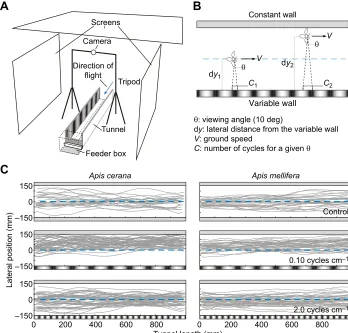
Biology, Lund University (55°43′N, 13°12′E), Sweden. A sucrose feeder (28 cm long, 5 cm wide and 4 cm deep) in a white plastic box was placed at the end of a plywood experimental tunnel (200 cm long, 30 cm wide, 30 cm high) behind a 15-cm-high vertical white plastic sheet, such that it was not visible to bees flying towards it (Fig. 1A). The tunnel floor was lined with white matte laminated paper, the top was covered with netting and the walls displayed different patterns (see below). To create a uniform light intensity along the length of the tunnel, it was shaded by a white cotton cloth (Fig. 1A). The average luminance in the tunnel and surroundings was similar for the two species and across all trials (A. cerana: ∼1900±400 lx;A. mellifera:∼2000±1000 lx), with no flights being recorded at light intensities below 750 lx.
Initially, bees were trained to fly along the tunnel and collect sucrose solution by gradually moving the feeder from the entrance towards its final position at the end. The bees then returned to the hive with their sucrose reward. Within each 30 min experimental session, individual foragers would return to the feeder a maximum of 5–6 times. Bees were also allowed to fly through the tunnel for 30 min before each session. During this time, both tunnel walls displayed randomized check patterns to minimize potential effects of previous asymmetric test conditions or wall following (Serres et al., 2008) on flight behaviour in the subsequent experimental
session. Foragers flying through the tunnel towards the feeder were filmed at 50 frames s−1using a video camera (Sony HDR-CX730) mounted 150 cm above the tunnel.
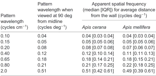
Estimation of spatial resolution and contrast thresholds During each experimental session, the‘constant wall’of the tunnel was uniformly grey while the‘variable wall’displayed one of the test gratings (Fig. 1). To estimate the highest spatial frequency that the bees can resolve, the variable wall displayed sinusoidal gratings of spatial wavelengths 0.10, 0.15, 0.20, 0.40, 0.65, 0.80 and 2.0 cycles cm−1, equivalent to spatial frequencies of 0.04, 0.05, 0.08, 0.12, 0.18, 0.21 and 0.51 cycles deg−1when seen from the midline of the tunnel (Table 1; distance to the variable wall dy1in Fig. 1B). These gratings had 87% Michelson contrast (MC; Michelson, 1927) determined as:
MC¼Imax Imin
Imax þ Imin : ð
1Þ
The intensity maximum (Imax) and intensity minimum (Imin) of the gratings were measured with a photometer (Hagner ScreenMaster, B. Hagner, Solna, Sweden) with the human photopic spectral sensitivity. To estimate the lowest visual contrast that bees could detect for a given spatial frequency, we used gratings with spatial frequencies of 0.10, 0.20 and 0.40 cycles cm−1, with Michelson contrasts of 87%, 39%, 22%, 14% and 3%.
The test gratings were presented in a pseudo-randomized order and equally often on the two walls. Thus, of the 50 flights analysed in each condition, 25 flights were filmed when the variable wall was
Tunnel length (mm)
Apis cerana Apis mellifera
Lateral position (mm) 150 150
–150 –150
0 0
0 200 400 600 800 0 200 400 600 800
150
–150 0
Control
0.10 cycles cm–1
2.0 cycles cm–1 dy2
C1 dy1
V
V
C2
θ
θ
θ: viewing angle (10 deg)
dy: lateral distance from the variable wall
V: ground speed
C: number of cycles for a given θ
A
B
C
Constant wall
Variable wall
Screens
Tripod
Tunnel
Feeder box Camera
[image:2.612.48.396.398.731.2]Direction of flight
Fig. 1. Experimental set-up and original flight paths of bees.(A) Schematic illustration of the experimental set-up. Honeybees were trained to enter the tunnel (blue arrow) and fly towards the feeder placed inside the feeder box. The trajectories were filmed using a camera mounted on a horizontal beam between two tripods. Screens on both sides and on top of the set-up were used to guarantee even illumination. The blue line shows the axis of the tunnel. (B) Illustration of parameters used in the analysis. (C) Flight tracks ofApis ceranaandApis melliferaflying through the middle section of a tunnel with two grey walls (control; top row), and tunnels with the variable wall displaying a low spatial frequency grating (0.10 cycles cm−1) and a high spatial frequency grating
(2.0 cycles cm−1). Note that the spatial frequency of the gratings is not to scale.
Journal
of
Experimental
on the right side and 25 flights when the variable wall was on the left side. The data for each condition were then pooled. As the control condition, both tunnel walls were covered with the uniform grey pattern, creating a symmetric situation, in which we filmed 25 flights.
Data analysis
The position of the bee was determined from each video frame over a distance of 100 cm in the middle section of the 200 cm long tunnel using an automated tracking program (Lindemann, 2005). Position data were converted from pixels to millimetres using a calibration pattern placed 15 cm above the tunnel floor (the approximate altitude of bees flying through the tunnel). Occasional flights that contained backward loops, crashes with the walls or other bees, or hovering by the top netting were excluded from the analysis. The lateral position of each bee with respect to the distance from the variable wall (y-position; dy2in Fig. 1B) was calculated for each frame and averaged for each flight. This value was also used to calculate the average perceived spatial frequency of the grating covering the variable wall as experienced by the bee during each flight.
Estimates of spatial resolution and contrast threshold were based on the assumption that bees could resolve/detect the grating presented on the variable wall when their lateral position and/or speed in an experimental condition differed significantly from the lateral position and speed in the control condition with two uniformly grey walls. Statistical tests were performed using ANOVA with Dunnet’s
post hocmultiple comparison test (Quinn and Keough, 2002).
RESULTS
The effect of spatial frequency on lateral position
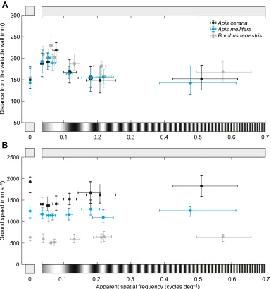
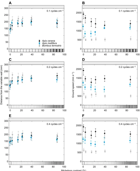
First, we tested how the lateral position of the bees varied with the spatial frequency of the sinusoidal grating presented on the variable wall while the constant wall was a uniform grey. Representative flight trajectories are shown in Fig. 1C, detailed results of all conditions are provided in Fig. 2A and statistics are presented in Table 2. In Fig. 2A, we present the mean lateral position of the bees as a function of the apparent spatial frequency, which depends on the bee’s distance to the variable wall (dy2, in Fig. 1B), and therefore differs slightly between species.
The mean lateral position of bothA. ceranaandA. melliferawas affected by the spatial frequency of the grating. Bees of both species flew further from the variable wall and closer to the constant wall when the grating had a spatial frequency of 0.10, 0.15 or 0.20 cycles cm−1. UnlikeA. cerana,A. melliferaalso appeared to fly closer to the constant wall when the grating had a spatial frequency of 0.4 cycles cm−1 (which corresponds to an apparent spatial frequency of 0.12 and 0.11 cycles deg−1, respectively; see
Table 2). At higher spatial frequencies, the bees instead flew along the midline of the tunnel, as they did in the control condition.
This result suggests that, as long as the bees could resolve the gratings, they flew farther from them in an attempt to balance the perceived magnitude of optic flow experienced in each eye. When they could no longer resolve the gratings, they perceived them as uniform grey (i.e. similar to the constant wall) and thus flew along the midline of the tunnel. Overall, these results indicate that, for directed forward flight,A. melliferahas a higher spatial resolution threshold (between 0.11 and 0.18 cycles deg−1 apparent spatial frequency) than A. cerana (between 0.08 and 0.12 cycles deg−1 apparent spatial frequency).
The effect of spatial frequency on ground speed
In the same flights as above,A. ceranaconsistently flew faster than
A. melliferathroughout all conditions (Fig. 2B). The ground speed
of both species was affected by spatial frequency, but the response to the different test conditions differed. When the spatial frequency of the grating on the variable wall was 0.65 or 2.0 cycles cm−1,
A. ceranaflew at the same speed as in the control condition, but for
all lower spatial frequencies, ground speed was significantly reduced. In contrast, ground speed in A. mellifera only differed significantly from the control condition in one experimental condition, when the grating had a spatial frequency of 0.2 cycles cm−1, but not with higher or lower spatial frequencies.
To further explore the effect of spatial frequency on ground speed, we also compared the data against the condition with the lowest spatial frequency (0.10 cycles cm−1, or 0.04 cycles deg−1 apparent spatial frequency; see Table 2), which both species could resolve. In
A. cerana, we found that ground speed was the same for spatial
frequencies of 0.4 cycles cm−1or lower, indicating that ground speed is not affected by spatial frequency for gratings that can be resolved.
InA. mellifera, this comparison once again showed that ground speed
does not vary significantly between spatial frequencies except for 0.65 cycles cm−1, when the bees flew slightly faster.
The effect of contrast on lateral position
Next, we investigated the effect of contrast on the lateral position of the bees. For these experiments, we used gratings of 0.10, 0.20 or 0.40 cycles cm−1at five different contrasts. Detailed results of all conditions are provided in Tables 3 and 4, and Fig. 3. The results suggest that contrast affected lateral position for all tested spatial frequencies in both species. ForA. cerana, lateral position did not differ from the control condition at 3% contrast at 0.10 cycles cm−1 and at 3% and 14% contrast at 0.40 cycles cm−1(Table 3, Fig. 3A, C,E), suggesting that they perceived these test gratings as grey. Under all other conditions, A. ceranaflew closer to the constant wall. This suggests that the contrast sensitivity forA. ceranalies somewhere between 7 and 33 for 0.10 cycles cm−1, is higher than 33 for 0.20 cycles cm−1 and lies between 4.5 and 7 for 0.40 cycles cm−1. For A. mellifera, lateral position differed significantly from the control in all conditions apart from 3% contrast at 0.40 cycles cm−1, suggesting a contrast sensitivity higher than 33 for 0.10 and 0.20 cycles cm−1, and between 7 and 33 for 0.40 cycles cm−1 (Tables 3 and 4, Fig. 3A,C,E). Taken together, these results suggest that A. mellifera in general have a higher contrast sensitivity thanA. cerana.
The effect of contrast on ground speed
Overall, contrast affected ground speed in both A. cerana and
A. melliferaat all tested spatial frequencies. Once again, however, the
[image:3.612.47.300.70.194.2]effect differed between the species (Tables 3 and 4, Fig. 3B). In all Table 1. Apparent spatial frequencies of sinusoidal gratings
Pattern wavelength (cycles cm−1)
Pattern
wavelength when viewed at 90 deg from midline (cycles deg−1)
Apparent spatial frequency (median [IQR]) for average distance
from the wall (cycles deg−1)
Apis cerana Apis mellifera
0.10 0.04 0.04 [0.03 0.04] 0.04 [0.03 0.04] 0.15 0.05 0.05 [0.05 0.06] 0.05 [0.05 0.06] 0.20 0.08 0.08 [0.07 0.08] 0.07 [0.06 0.07] 0.40 0.12 0.12 [0.10 0.14] 0.11 [0.11 0.13] 0.65 0.18 0.18 [0.14 0.21] 0.18 [0.15 0.21] 0.80 0.21 0.21 [0.17 0.25] 0.22 [0.18 0.25] 2.0 0.51 0.51 [0.42 0.61] 0.49 [0.39 0.61]
IQR, interquartile range.
Journal
of
Experimental
test conditions,A. ceranawas flying at a significantly lower ground speed than in the control. However, when comparing against flights with 87% contrast for each spatial frequency, only ground speed in the control (0% contrast) and 3% contrast at 0.10 cycles cm−1 was significantly higher (Table 4), suggesting that differences in contrast above 3% have little effect on ground speed inA. cerana.
For A. melliferaat 0.1 cycles cm−1, however, ground speed was
significantly lower than the control at 3%, 14% and 22% contrast but increased to control levels at 39% and 87%. At 0.20 cycles cm−1, ground speed was lower than the control for all contrasts and at 0.40 cycles cm−1, it was lower than the control for all contrasts except 3% and 87%.
DISCUSSION
We investigated the spatial resolution and contrast dependency of the visual system regulating flight control in two closely related honeybee species,A. cerana andA. mellifera. Overall, we found that spatial frequency and contrast do affect position control and
ground speed in both species although the specific responses are surprisingly different.
Apis melliferahas a higher spatial resolution for flight control thanA. cerana, but lower than that ofB. terrestris
Our results suggest that the spatial resolution limit of visual flight control in A. cerana lies between 0.08 and 0.12 cycles deg−1 while the spatial resolution limit for A. mellifera appears to be slightly higher, lying between 0.11 and 0.18 cycles deg−1. These results represent conservative estimates as they are based upon measurements of the spatial frequency of the gratings as they would appear in the lateral field of view. If the bees are measuring optic flow for flight control in more frontal visual areas, as bumblebees do (Baird et al., 2010; Linander et al., 2015), then these limits would be even higher. For example, if the bees measure optic flow at a 45 deg angle frontally, these values become more similar to the estimate of maximal resolution obtained with two gratings in a dual-choice test (see Table 5): 0.26–0.36 cycles deg−1forA. cerana(Zhang et al.,
0 0.1 0.2 0.3 0.4 0.5 0.6 0.7
0 500 1000 1500 2000 2500
Ground speed (mm s
–1
)
0 0.1 0.2 0.3 0.4 0.5 0.6 0.7
Apparent spatial frequency (cycles deg–1) 50
100 150 200 250 300
Distance from the variable wall (mm)
Apis cerana Apis mellifera Bombus terrestris
A
[image:4.612.116.501.58.468.2]B
Fig. 2. Effect of apparent spatial frequency of gratings on the variable wall of a tunnel on the lateral position and ground speed ofA. cerana,A. mellifera andBombus terrestris.(A) Lateral position (calculated as the average distance to the variable wall) as a function of the average apparent spatial frequency of the grating. Circles give the median apparent spatial frequency and lateral position, whiskers represent the second and third quartiles. (B) Ground speed at the apparent spatial frequency of the grating. Circles give the median apparent spatial frequency and ground speed, whiskers the second and third quartiles. See Table 2 for statistics. Data onB. terrestrisfrom Chakravarthi et al. (2017). Note that the spatial frequency of the gratings is not to scale.
Journal
of
Experimental
2014) and 0.25 cycles deg−1 for A. mellifera (Srinivasan and Lehrer, 1988).
The smallest high-contrast objects that A. mellifera could be trained to detect from a background were circular discs with a diameter of 3 deg (Lehrer and Bischof, 1995), which would translate into a spatial frequency of merely 0.17 cycles deg−1, similar to the resolution threshold found in our study forA. mellifera(Table 5). Subsequent studies have estimated the detection threshold for circular stimuli to lie between 3.7 and 5 deg (Giurfa et al., 1996; Giurfa and Vorobyev, 1998; Hempel de Ibarra et al., 2001; Wertlen et al., 2008; see Table 5), possibly because they used targets with lower achromatic contrast to the background.
For both species, the behaviourally measured limits of spatial resolution presented in this and earlier studies are coarser than the anatomically estimated limits (using acceptance angles): ∼0.8 cycles deg−1 for A. cerana (Somanathan et al., 2009) and ∼0.6 cycles deg−1forA. mellifera(Greiner et al., 2004); however, these are values obtained for the frontal visual field. The average acceptance angles of light-adapted photoreceptors looking at the horizon in
A. melliferahave recently been determined electrophysiologically as
2.5 and 1.9 deg in the lateral and frontal visual fields, respectively (full width at half maximum; Rigosi et al., 2017), translating into a potential spatial resolution limit of 0.4 cycles deg−1in the lateral visual field and 0.5 cycles deg−1in the frontal visual field. The difference between the electrophysiologically and the behaviourally determined resolution could be explained by the fact that small objects (below the spatial resolution threshold) still elicit a response because of the high contrast
sensitivity of the photoreceptors, rather than the actual angular size of the object (O’Carroll and Wiederman, 2014). Complex behaviours, however, like flower searching, require supra-threshold stimuli seen in more than one ommatidium (Giurfa et al., 1996; Hempel de Ibarra et al., 2001), leading to a lower resolution.
The finding that flight control has coarser spatial resolution than the anatomically or physiologically defined limits is consistent with the conclusions of a similar study performed in the bumblebee,
B. terrestris(Chakravarthi et al., 2017). In this species, the limit of
spatial resolution for flight control was estimated at 0.21 cycles deg−1, while the anatomical estimation (using interommatidial angles; Spaethe and Chittka, 2003) was 0.55 cycles deg−1. It is also interesting to note that, for the gratings that the bumblebees could resolve, they generally flew further away from the wall bearing the grating than either honeybee species tested here (see grey data points in Fig. 3A,C,E, taken from Chakravarthi et al., 2017). This finding suggests that not only do bees of different species have different limits of spatial resolution for flight control but also the strength of their flight control behaviour appears to vary.
Apis melliferaandB. terrestrishave higher contrast sensitivity for flight control thanA. cerana
For one spatial frequency (0.2 cycles cm−1 or 0.08 cycles deg−1),
A. ceranahad a contrast sensitivity above 33 (the inverse of contrast
threshold, in this case 3%) but for both higher and lower spatial frequencies, contrast sensitivity was lower. The contrast sensitivity of
[image:5.612.48.565.71.411.2]A. mellifera, however, was above 33 for all frequencies except for the
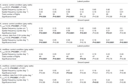
Table 2. Effect of spatial frequency on lateral position and ground speed ofApis ceranaandApis mellifera
Lateral position
A. cerana: control condition (grey walls)
F7,438=25.51;P<0.0001;na=446
Spatial frequency (cycles cm−1) 0.10 0.15 0.20 0.40 0.65 0.80 2.0
Spatial frequency (cycles deg−1) 0.04 0.05 0.08 0.12 0.18 0.21 0.51
Total number of flights 50 50 75 50 51 95 50
Significance level P=0.004 P<0.0001 P<0.0001 P=0.25 P>0.99 P>0.99 P>0.99 Ground speed
A. cerana: control condition (grey walls)
F7,438=14.50;P<0.0001;nb=446
Spatial frequency (cycles cm−1) 0.10 0.15 0.20 0.40 0.65 0.80 2.0
Spatial frequency (cycles deg−1) 0.04 0.05 0.08 0.12 0.18 0.21 0.51
Significance level P<0.0001 P<0.0001 P<0.0001 P=0.001 P=0.09 P=0.01 P>0.99
A. cerana: data from 0.04 cycles deg−1
F7,438=14.50;P<0.0001;nb=446
Spatial frequency (cycles deg−1) Grey 0.05 0.08 0.12 0.18 0.21 0.51
Significance level P<0.0001 P>0.99 P>0.99 P=0.16 P<0.0001 P<0.0001 P<0.0001 Lateral position
A. mellifera: control condition (grey walls)
F7,343=20.54;P<0.0001;na=351
Spatial frequency (cycles deg−1) 0.04 0.05 0.07 0.11 0.18 0.22 0.49
Total number of flights 49 54 46 43 47 44 39
Significance level P<0.0001 P<0.0001 P<0.0001 P=0.04 P=0.90 P=0.78 P>0.99
Ground speed
A. mellifera: control condition (grey walls)
F7,343=5.15;P<0.0001;na=351
Spatial frequency (cycles deg−1) 0.04 0.05 0.07 0.11 0.18 0.22 0.49
Significance level P=0.84 P=0.26 P=0.02 P=0.84 P=0.4 P=0.15 P>0.99
A. mellifera: data from 0.04 cycles deg−1
F7,343=5.15;P<0.0001;na=351
Spatial frequency (cycles deg−1) Grey 0.05 0.07 0.11 0.18 0.22 0.49
Significance level P=0.89 P=0.86 P=0.13 P>0.99 P=0.02 P=0.63 P=0.80 Data were obtained by ANOVA with Dunnet’spost hocmultiple comparison for the conditions shown.
aTotal number of flights (including the control data,n=25) analysed.bTotal number of flights (including the control data,n=29) analysed.
Journal
of
Experimental
highest tested frequency, 0.4 cycles cm−1(0.12 cycles deg−1). These results are consistent with free-flight experiments onA. melliferathat found no effect of reducing the contrast of square-wave gratings down to 15% (Srinivasan et al., 1991) or 10% (Baird et al., 2005) on lateral position and speed control, respectively.
In experiments similar to those conducted here, the bumblebee
B. terrestris was also found to have a peak contrast sensitivity
greater than 33 for a broad range of spatial frequencies, suggesting that the motion detection systems underlying flight control in bees generally have very high contrast sensitivity. In a second species of bumblebee,Bombus impatiens, only patterns with 5% contrast have been tested, and only for a single spatial frequency (0.03 cycles deg−1), resulting in an estimate of at least 20 for their contrast sensitivity (Dyhr and Higgins, 2010).
Spatial contrast sensitivity has also been estimated in discrimination tasks. In dual-choice tests with vertical and
horizontal square-wave gratings, A. mellifera could detect 8% contrast at 0.09 cycles deg−1, equivalent to a contrast sensitivity of at least 12.5 (Srinivasan and Lehrer, 1988), but the threshold was not determined. In a similar paradigm,B. terrestriswas found to have a contrast sensitivity of 1.57 (64% contrast; Chakravarthi et al., 2016), which is much lower than that measured for flight control in the same species (Chakravarthi et al., 2017), but experimental conditions may have contributed to this low value (Chakravarthi et al., 2016).
[image:6.612.48.569.69.527.2]High contrast sensitivity for moving stimuli is a general property of insect vision. In A. mellifera, reactions to stimuli as small as 0.6×0.6 deg have been recorded electrophysiologically in the frontal visual field and 0.75×0.75 deg in the lateral visual field (Rigosi et al., 2017). This leads to an estimation of the lowest contrast that can be detected by single photoreceptors of laterally looking ommatidia of A. mellifera of around 9% (Rigosi et al., 2017).
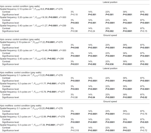
Table 3. Effect of contrast on lateral position and ground speed inApis ceranaandApis mellifera
Lateral position
Apis cerana: control condition (grey walls) Spatial frequency: 0.10 cycles cm−1;F
5,269=8.6;P<0.0001;na=275
Contrast 3% 14% 22% 39% 87%
Significance level P=0.18 P=0.001 P=0.001 P<0.0001 P=0.002
Spatial frequency: 0.20 cycles cm−1;F
5,294=16.39;P<0.0001;na=300
Contrast 3% 14% 22% 39% 87%
Significance level P=0.003 P=0.001 P<0.0001 P<0.0001 P<0.0001 Spatial frequency: 0.40 cycles cm−1;F
5,293=11.27;P<0.0001;na=299
Contrast 3% 14% 22% 39% 87%
Significance level P=0.98 P=0.24 P=0.002 P<0.0001 P=0.15
Ground speed
Apis cerana: control condition (grey walls) Spatial frequency: 0.10 cycles cm−1;F
5,269=17.22;P<0.0001;na=275
Contrast 3% 14% 22% 39% 87%
Significance level P=0.048 P<0.0001 P<0.0001 P<0.0001 P<0.0001 Spatial frequency: 0.20 cycles cm−1;F
5,294=15.46;P<0.0001;na=300
Contrast 3% 14% 22% 39% 87%
Significance level P<0.0001 P<0.0001 P<0.0001 P<0.0001 P<0.0001 Spatial frequency: 0.40 cycles cm−1;F
5,293=3.82;P=0.002;na=299
Contrast 3% 14% 22% 39% 87%
Significance level P=0.031 P=0.002 P=0.036 P<0.0001 P=0.002
Lateral position
Apis mellifera: control condition (grey walls) Spatial frequency: 0.1 cycles cm−1;F
5,272=13.20;P<0.0001;nb=278
Contrast 3% 14% 22% 39% 87%
Significance level P<0.0001 P<0.0001 P<0.0001 P<0.0001 P<0.0001 Spatial frequency: 0.2 cycles cm−1;F
5,272=11.77;P<0.0001;nb=278
Contrast 3% 14% 22% 39% 87%
Significance level P=0.003 P<0.0001 P<0.0001 P<0.0001 P<0.0001 Spatial frequency: 0.4 cycles cm−1;F
5,271=10.76;P<0.0001;nb=277
Contrast 3% 14% 22% 39% 87%
Significance level P=0.98 P=0.04 P<0.0001 P<0.0001 P=0.02
Ground speed
Apis mellifera: control condition (grey walls) Spatial frequency: 0.1 cycles cm−1;F
5,272=33.20;P<0.0001;nb=278
Contrast 3% 14% 22% 39% 87%
Significance level P<0.0001 P<0.0001 P<0.0001 P=0.63 P=0.76 Spatial frequency: 0.2 cycles cm−1;F
5,272=12.89;P<0.0001;nb=278
Contrast 3% 14% 22% 39% 87%
Significance level P<0.0001 P<0.0001 P<0.0001 P<0.0001 P=0.025 Spatial frequency: 0.4 cycles cm−1;F
5,271=7.39;P<0.0001;nb=277
Contrast 3% 14% 22% 39% 87%
Significance level P=0.318 P<0.0001 P<0.0001 P=0.021 P=0.72
Data were obtained by ANOVA with Dunnet’spost hocmultiple comparison for the conditions shown. Bold indicates significance. aTotal number of analysed flights (including the control data,n=25).bTotal number of analysed flights (including the control data,n=29).
Journal
of
Experimental
However, because the signals from six photoreceptors in one ommatidium converge onto the neurons in the next optic neuropil– a system that reduces noise by the square root of 6–the contrast sensitivity at later processing stages in the visual system is likely to be higher, with a threshold closer to 4% (equating to a contrast sensitivity of 25; see Rigosi et al., 2017). The bees in the present study were probably using information coming from a wide field of view involving many ommatidia. This could further enhance the signal-to-noise ratio and, with it, contrast sensitivity, thereby explaining the minimum value of 33 recorded in the present study for both A. cerana and A. mellifera. The electrophysiologically determined contrast sensitivity of wide-field motion-sensitive neurons in the optic lobe of A. mellifera of ∼30 for moving grating lies within a similar range (Bidwell and Goodman, 1993). Generally, wide-field motion-sensitive neurons of insects including butterflies, flies and hawkmoths have been shown to have contrast sensitivities between 20 and 100 (Dvorak et al., 1980; Maddess et al., 1991; O’Caroll et al., 1996; Stöckl et al., 2016; O’Caroll and Wiederman, 2014).
Ground speed and its response to changes in spatial frequency and contrast differ between species
While the effect of spatial frequency and contrast on position control was similar acrossA. cerana,A. melliferaandB. terrestris, it is notable that the effect of these variables on ground speed varied between the species. For low spatial frequencies, A. ceranaflew slower in comparison to the control condition but increased its speed when–according to lateral position data–it could no longer resolve the gratings. Conversely, spatial frequency had no systematic effect on speed inA. mellifera. This is consistent with the findings of Baird et al. (2005). These results withA. mellifera are similar to those found in bumblebees B. terrestris, using the same experimental paradigm as the present study (Chakravarthi et al., 2017).
Variations in the effect of spatial frequency on flight control observed across the species do not appear to be related to the actual speed at which the bees fly becauseA. melliferaflew approximately twice as fast asB. terrestrisandA. ceranaflew between 200 and
1000 mm s−1faster thanA. mellifera(Fig. 3B,D,F). These general differences in speed responses were also present in the control condition, where median ground speed was 632 mm s−1 in
B. terrestris, 1244 mm s−1 in A. mellifera and 1927 mm s−1 in
A. cerana(see Fig. 2B). This indicates that, even in the presence of
weak optic flow cues, each of these species appears to have different preferred set-points for speed control.
Differences in speed response between the species were also observed when the grating contrast changed.Apis ceranatended to fly faster when the grating was or appeared to be grey than when they could detect the contrast – in which case, speed remained constant.Apis melliferaalso tended to fly faster when the grating was or appeared to be grey but decreased its speed for the lower detectable contrasts, before flying faster again. We found this difference in ground speed response to contrast intriguing so, to better understand it, we calculated the speed response for the same conditions inB. terrestrisusing data from Chakravarthi et al. (2017). Interestingly, we found yet another response to differences in contrast.Bombus terrestrisappeared not to change their speed in any systematic manner in response to changes in contrast. It is quite surprising that these three species all display different speed responses to changes in grating contrast, particularly the closely relatedA. ceranaandA. mellifera, while their position responses are very similar. Behavioural differences between these two species have also been recorded with respect to their foraging ranges–with
A. melliferahaving a larger range thanA. cerana(He et al., 2012)–
and with respect to their learning and memory performance –
with A. ceranabeing superior toA. mellifera (Qin et al., 2012).
While there is no obvious explanation for these differences given that these species can occupy the same ecological niche and are morphologically very similar (Somanathan et al., 2009), some clues might arise from exploring their physiological and anatomical bases.
[image:7.612.50.564.68.279.2]These findings suggest that position and speed control may be regulated by different systems of motion vision in these species, something that was also suggested for B. terrestris by Linander et al. (2015). Although the basis of these differences is not clear, this result highlights the fact that ground speed control can vary
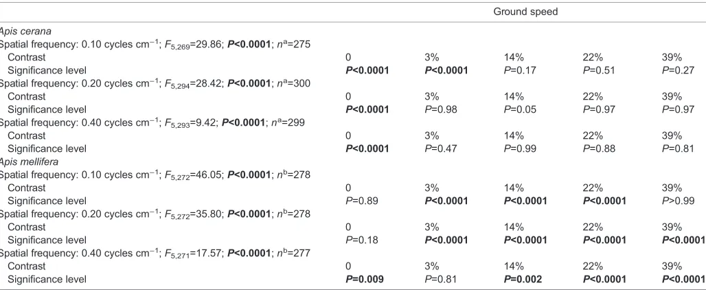
Table 4. Effect of contrast on ground speed ofApis ceranaandApis melliferacompared with patterns with 87% contrast
Ground speed
Apis cerana
Spatial frequency: 0.10 cycles cm−1;F
5,269=29.86;P<0.0001;na=275
Contrast 0 3% 14% 22% 39%
Significance level P<0.0001 P<0.0001 P=0.17 P=0.51 P=0.27
Spatial frequency: 0.20 cycles cm−1;F
5,294=28.42;P<0.0001;na=300
Contrast 0 3% 14% 22% 39%
Significance level P<0.0001 P=0.98 P=0.05 P=0.97 P=0.97
Spatial frequency: 0.40 cycles cm−1;F
5,293=9.42;P<0.0001;na=299
Contrast 0 3% 14% 22% 39%
Significance level P<0.0001 P=0.47 P=0.99 P=0.88 P=0.81
Apis mellifera
Spatial frequency: 0.10 cycles cm−1;F
5,272=46.05;P<0.0001;nb=278
Contrast 0 3% 14% 22% 39%
Significance level P=0.89 P<0.0001 P<0.0001 P<0.0001 P>0.99 Spatial frequency: 0.20 cycles cm−1;F
5,272=35.80;P<0.0001;nb=278
Contrast 0 3% 14% 22% 39%
Significance level P=0.18 P<0.0001 P<0.0001 P<0.0001 P<0.0001 Spatial frequency: 0.40 cycles cm−1;F
5,271=17.57;P<0.0001;nb=277
Contrast 0 3% 14% 22% 39%
Significance level P=0.009 P=0.81 P=0.002 P<0.0001 P<0.0001
Data were obtained by ANOVA with Dunnet’spost hocmultiple comparison with 87% contrast. Bold indicates significance. aTotal no. of analysed flights (including the control data,n=25).bTotal no. of analysed flights (including the control data,n=29).
Journal
of
Experimental
radically between insect species and that findings from one species cannot necessarily be generalized to others. More systematic and detailed comparative studies in other insect species would be fruitful in understanding how wide-spread such differences are.
Concluding remarks
The aim of the present study was to further explore the limits of visually guided behaviour in insects by describing the spatial resolution and contrast sensitivity limits of visually guided flight control in the honeybeesA. ceranaandA. mellifera.
Apis cerana Apis mellifera Bombus terrestris
0 50 100 150 200 250 300
0 50 100 150 200 250 300
Distance from the variable wall (mm)
0 50 100 150 200 250 300
0 20 40 60 80 100 0 20 40 60 80 100
0 20 40 60 80 100 0 20 40 60 80 100
0 20 40 60 80 100 0 20 40 60 80 100
Michelson contrast (%) 0 500 1000 1500 2000
0 500 1000 1500 2000
Ground speed (mm s
–1
)
0 500 1000 1500 2000 0.1 cycles cm–1
0.2 cycles cm–1
0.4 cycles cm–1
0.1 cycles cm–1
0.2 cycles cm–1
0.4 cycles cm–1
A
C
E
B
D
[image:8.612.77.536.55.617.2]F
Fig. 3. Effect of the contrast of gratings on the variable wall of a tunnel on the lateral position and ground speed ofA. cerana,A. melliferaand B. terrestris.Lateral position (A,C,E) and ground speed (B,D,F) as a function of the Michelson contrast of the grating. Circles give the median apparent spatial frequency and lateral position, whiskers represent the second and third quartiles. Results with grating with 0.10, 0.20 and 0.40 cycles cm−1(from top to bottom) are shown. See Tables 3 and 4 for statistics. Data onB. terrestrisfrom Chakravarthi et al. (2017). Note that the spatial frequency and contrast of the gratings are not to scale.
Journal
of
Experimental
Our results show that the system mediating flight control inA.
ceranaandA. melliferahas a low resolution when compared with
the anatomical estimate and is also potentially lower than the system mediating object detection, but that it is sensitive to very low contrasts. Based on the lateral position (Table 2) and ground speed (Tables 3 and 4) data, the contrast sensitivity inA. ceranapeaks at the intermediate spatial frequency of 0.20 cycles cm−1and drops off at the lowest and highest spatial frequency tested, showing a band pass-like function (De Valois and De Valois, 1990). Low resolution and high contrast sensitivity are well suited for extracting wide-field optic flow information (Srinivasan and Bernard, 1975). It can be seen that the resolution determined for an object discrimination task when compared with position control is higher by an approximate factor of 2. This is in agreement with the prediction that translational optic flow is optimally sampled with low resolution and high contrast sensitivity (Srinivasan and Bernard, 1975), and similar observations have also been reported for birds (Haller et al., 2014) and humans (Robson, 1966; Barten, 1993). Thus, a bee flying over a meadow can use low-resolution information to avoid crashing into obstacles but can still resolve the flowers or food sources she approaches to find nectar and pollen. Future investigations into the limits of insect vision should test the animals under several behavioural tasks and take into account the visual field being used for them if we are to thoroughly understand the limitations of their visually guided behaviour.
Acknowledgements
We are grateful to Sannuvanda K. Chengappa for help with setting up experiments, to Ramprasad Rao for maintainingA. ceranacolonies and to Dhiraj Bhaisare of ARRS for logistics. We thank Hema Somanathan, Balamurali G. S. and Asna (IISER Thiruvananthapuram) for support during pilot experiments. We are grateful to Helena Kelber and Morgan Brain for help with field work and video processing, to
Lana Khaldy, Lina O’Reilly and Therese Reber for help in digitizing videos, to Gavin Taylor and Jochen Smolka for Matlab codes and to Lars Råberg for statistical advice.
Competing interests
The authors declare no competing or financial interests.
Author contributions
Conceptualization: A.C., A.K., M.D., E.B.; Methodology: A.C., A.K., M.D., E.B.; Software: E.B.; Validation: A.K., E.B.; Formal analysis: A.C., S.R., E.B.; Investigation: A.C., S.R., E.B.; Resources: A.K., M.D., E.B.; Data curation: A.C., E.B.; Writing - original draft: A.C., A.K., M.D., E.B.; Writing - review & editing: A.C., A.K., M.D., E.B.; Visualization: A.C., E.B.; Supervision: A.K., M.D., E.B.; Project administration: A.K., M.D.; Funding acquisition: A.K., M.D., E.B.
Funding
Financial support from the Knut and Alice Wallenberg Foundation (Knut och Alice Wallenbergs Stiftelse), and the Swedish Research Council (Vetenskapsrådet; grants 2011-4701, 2012-2212 and 2014-4762) is gratefully acknowledged.
Data availability
Data have been deposited in the Dryad Digital Repository (Chakravarthi et al., 2018): doi:10.5061/dryad.n0vr7d0.
References
Baird, E., Srinivasan, M. V., Zhang, S. and Cowling, A.(2005). Visual control of flight speed in honeybees.J. Exp. Biol.208, 3895-3905.
Baird, E., Kornfeldt, T. and Dacke, M.(2010). Minimum viewing angle for visually guided ground speed control in bumblebees. J. Exp. Biol.213, 1625-1632.
Barten, P. G. J.(1993). Spatio-temporal model for the contrast sensitivity of the human eye and its temporal aspects. In Human Vision, Visual Processing, and Digital Display IV. Proc. SPIE 1913, 2-14.
Baumgärtner, H.(1928). Der Formensinn und die Sehschärfe der Bienen.Z. Vergl.
Physiol.7, 56-143.
Bidwell, N. J. and Goodman, L. J.(1993). Possible functions of a population of descending neurons in the honeybee’s visuo-motor pathway.Apidologie24, 333-354.
Chakravarthi, A., Baird, E., Dacke, M. and Kelber, A.(2016). Spatial vision in
[image:9.612.46.560.73.364.2]Bombus terrestris.Front. Behav. Neurosci.10, 17.
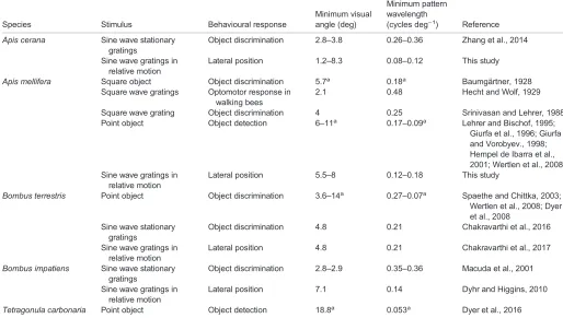
Table 5. Behaviourally determined thresholds of spatial resolution in bees
Species Stimulus Behavioural response
Minimum visual angle (deg)
Minimum pattern wavelength
(cycles deg−1) Reference
Apis cerana Sine wave stationary gratings
Object discrimination 2.8–3.8 0.26–0.36 Zhang et al., 2014
Sine wave gratings in relative motion
Lateral position 1.2–8.3 0.08–0.12 This study
Apis mellifera Square object Object discrimination 5.7a 0.18a Baumgärtner, 1928 Square wave gratings Optomotor response in
walking bees
2.1 0.48 Hecht and Wolf, 1929
Square wave grating Object discrimination 4 0.25 Srinivasan and Lehrer, 1988 Point object Object detection 6–11a 0.17–0.09a Lehrer and Bischof, 1995;
Giurfa et al., 1996; Giurfa and Vorobyev., 1998; Hempel de Ibarra et al., 2001; Wertlen et al., 2008 Sine wave gratings in
relative motion
Lateral position 5.5–8 0.12–0.18 This study
Bombus terrestris Point object Object discrimination 3.6–14a 0.27–0.07a Spaethe and Chittka, 2003; Wertlen et al., 2008; Dyer et al., 2008
Sine wave stationary gratings
Object discrimination 4.8 0.21 Chakravarthi et al., 2016
Sine wave gratings in relative motion
Lateral position 4.8 0.21 Chakravarthi et al., 2017
Bombus impatiens Sine wave stationary gratings
Object discrimination 2.8–2.9 0.35–0.36 Macuda et al., 2001
Sine wave gratings in relative motion
Lateral position 7.1 0.14 Dyhr and Higgins, 2010
Tetragonula carbonaria Point object Object detection 18.8a 0.053a Dyer et al., 2016
aValues were calculated considering the visual angle of a single object as half the resolvable wavelength. A full cycle of an equivalent grating would be twice the angle of the single object.
Journal
of
Experimental
Chakravarthi, A., Kelber, A., Baird, E. and Dacke, M.(2017). High contrast sensitivity for visually guided flight control in bumblebees.J. Comp. Physiol. A
203, 999-1006.
Chakravarthi, A., Rajus, S., Kelber, A., Dacke, M. and Baird, E.(2018). Data from: Differences in spatial resolution and contrast sensitivity of flight control in the honeybeesApis ceranaandApis mellifera.Dryad Digital Repository. https://doi. org/10.5061/dryad.n0vr7d0
De Valois, R. L. and De Valois, K. K.(1990).Spatial Vision. New York: Oxford University Press.
Dvorak, D. R., Srinivasan, M. V. and French, A. S.(1980). The contrast sensitivity of fly movement-detecting neurons.Vis. Res.20, 397-407.
Dyer, J. P., Spaethe, J. and Prack, S.(2008). Comparative psychophysics of bumblebee and honeybee colour discrimination and object detection.J. Comp.
Physiol. A194, 617-627.
Dyer, A. G., Streinzer, M. and Garcia, J.(2016). Flower detection and acuity of the Australian native stingless beeTetragonula carbonariaSm.J. Comp. Physiol. A
202, 629-639.
Dyhr, J. P. and Higgins, C. M.(2010). The spatial frequency tuning of optic-flow-dependent behaviors in the bumblebeeBombus impatiens.J. Exp. Biol.213, 1643-1650.
Giurfa, M. and Vorobyev, M.(1998). The angular range of achromatic target detection by honey bees.J. Comp. Physiol. A183, 101-110.
Giurfa, M., Vorobyev, M., Kevan, P. and Menzel, R.(1996). Detection of coloured stimuli by honeybees: minimum visual angles and receptor specific contrasts.
J. Comp. Physiol. A178, 699-709.
Greiner, B., Ribi, W. A. and Warrant, E. J.(2004). Retinal and optical adaptations for nocturnal vision in the halictid beeMegalopta genalis.Cell Tissue Res.316, 377-390.
Haller, N. K., Lind, O., Steinlechner, S. and Kelber, A.(2014). Stimulus motion improves spatial contrast sensitivity in budgerigars (Melopsittacus undulatus).
Vision Res.102, 19-25.
He, X., Wang, W., Qin, Q., Zeng, Z., Zhang, S. W. and Barron, A.(2012). Assessment of flight activity and homing ability in Asian and European honey bee species,Apis ceranaandApis mellifera, measured with radio frequency tags.
Apidologie44, 38-51.
Hecht, S. and Wolf, E.(1929). The visual acuity of the honey bee.J. Gen. Physiol.
12, 727-760.
Hempel de Ibarra, N., Giurfa, M. and Vorobyev, M.(2001). Detection of coloured patterns by honeybees through chromatic and achromatic cues.J. Comp. Physiol. A187, 215-224.
Kelly, D. H. (1979). Motion and vision II: stabilized spatio-temporal threshold surface.J. Opt. Soc. Am.69, 1340-1349.
Land, M. F.(1997). Visual acuity in insects.Annu. Rev. Entomol.42, 147-177.
Lehrer, M. and Bischof, S.(1995). Detection of model flowers by honeybees: the role of chromatic and achromatic contrast.Naturwissenschaften82, 145-147.
Linander, N., Dacke, M. and Baird, E.(2015). Bumblebees measure optic flow for position and speed control flexibly within the frontal visual field.J. Exp. Biol.218, 1051-1059.
Lindemann, J.(2005). Visual navigation of a virtual blowfly.PhD thesis, Universität Bielefeld, Germany.
Macuda, T., Gegear, R. J., Laverty, T. M. and Timney, B.(2001). Behavioural assessment of visual acuity in bumblebees (Bombus impatiens).J. Exp. Biol.204, 559-564.
Maddess, T., Dubois, R. A. and Ibbotson, M. R.(1991). Response properties and adaptation of neurons sensitive to image motion in the butterflyPapilio aegeus.
J. Exp. Biol.161, 171-199.
Michelson, A. A.(1927).Studies in Optics. Chicago: The University of Chicago Press.
O’Carroll, D. C. and Wiederman, S. D. (2014). Contrast sensitivity and the detection of moving patterns and features.Philos. Trans. R. Soc. B 369, 20130043.
O’Carroll, D. C., Bidweii, N. J., Laughlin, S. B. and Warrant, E. J.(1996). Insect motion detectors matched to visual ecology.Nature382, 63-66.
Qin, Q.-H., He, X.-J., Tian, L.-Q., Zhang, S.-W. and Zeng, Z.-J.(2012). Comparison of learning and memory ofApis ceranaandApis mellifera.J. Comp. Physiol. A
198, 777-786.
Quinn, G. P. and Keough, M. J.(2002).Experimental Design and Data Analysis
for Biologists. Cambridge, UK: Cambridge University Press.
Rigosi, E., Wiederman, S. D. and O’Carroll, D. C.(2017). Visual acuity of the honey bee retina and the limits for feature detection.Sci. Rep.7, 45972.
Robson, J. G.(1966). Spatial and temporal contrast-sensitivity functions of the visual system.J. Opt. Soc. Am.56, 1141-1142.
Serres, J. R., Masson, G. P., Ruffier, F. and Franceschini, N. (2008). A bee in the corridor: centering and wall-following.Naturwissenschaften 95, 1181-1187.
Somanathan, H., Warrant, E. J., Borges, R. M., Wallen, R. and Kelber, A.(2009). Resolution and sensitivity of the eyes of the Asian honeybeesApis florea, Apis
ceranaandApis dorsata.J. Exp. Biol.212, 2448-2453.
Spaethe, J. and Chittka, L.(2003). Interindividual variation of eye optics and single object resolution in bumblebees.J. Exp. Biol.206, 3447-3453.
Srinivasan, M. V. and Bernard, G. D.(1975). The effect of motion on visual acuity of the compound eye: a theoretical analysis.Vis. Res.15, 515-525.
Srinivasan, M. V. and Lehrer, M.(1988). Spatial acuity of honeybee vision and its spectral properties. J. Comp. Physiol. A162, 159-172.
Srinivasan, M. V., Lehrer, M., Kirchner, W. H. and Zhang, S. W.(1991). Range perception through apparent image speed in freely flying honeybees. Vis.
Neurosci.6, 519-535.
Srinivasan, M. V., Zhang, S., Lehrer, M. and Collett, T. (1996). Honeybee navigation en route to the goal: visual flight control and odometry.J. Exp. Biol.199, 237-244.
Stavenga, D. G.(2003). Angular and spectral sensitivity of fly photoreceptors. II. Dependence on facet lens F- number and rhabdomere type inDrosophila.
J. Comp. Physiol. A189, 189-202.
Stavenga, D. G.(2004). Angular and spectral sensitivity of fly photoreceptors. III. Dependence on the pupil mechanism in the blowflyCalliphora.J. Comp. Physiol. A190, 115-129.
Stöckl, A. L., O’Carroll, D. C. and Warrant, E. J.(2016). Neural summation in the hawkmoth visual system extends the limits of vision in dim light. Curr. Biol.26, 821-826.
Uhlrich, D. J., Essock, E. A. and Lehmkuhle, S. (1981). Cross-species correspondence of spatial contrast sensitivity functions.Behav. Brain Res.2, 291-299.
Warrant, E. J., Kelber, A. and Frederiksen, R.(2007). Ommatidial adaptations for spatial, spectral and polarisation vision in arthropods. In Invertebrate
Neurobiology(ed. G. North and R. Greenspan), pp. 123-154. Woodbury: Cold
Spring Harbor Laboratory Press.
Wertlen, A. M., Niggebrügge, C., Vorobyev, M. and Hempel de Ibarra, N.
(2008). Detection of patches of coloured discs by bees. J. Exp. Biol. 211, 2101-2104.
Zhang, L.-Z., Zhang, S.-W., Wang, Z.-L., Yan, W.-Y. and Zeng, Z.-J.(2014). Cross-modal interaction between visual and olfactory learning inApis cerana.
J. Comp. Physiol. A200, 899-909.