warwick.ac.uk/lib-publications
Manuscript version: Author’s Accepted Manuscript
The version presented in WRAP is the author’s accepted manuscript and may differ from the
published version or Version of Record.
Persistent WRAP URL:
http://wrap.warwick.ac.uk/116198
How to cite:
Please refer to published version for the most recent bibliographic citation information.
If a published version is known of, the repository item page linked to above, will contain
details on accessing it.
Copyright and reuse:
The Warwick Research Archive Portal (WRAP) makes this work by researchers of the
University of Warwick available open access under the following conditions.
Copyright © and all moral rights to the version of the paper presented here belong to the
individual author(s) and/or other copyright owners. To the extent reasonable and
practicable the material made available in WRAP has been checked for eligibility before
being made available.
Copies of full items can be used for personal research or study, educational, or not-for-profit
purposes without prior permission or charge. Provided that the authors, title and full
bibliographic details are credited, a hyperlink and/or URL is given for the original metadata
page and the content is not changed in any way.
Publisher’s statement:
Please refer to the repository item page, publisher’s statement section, for further
information.
arXiv:1311.5806v2 [cs.DC] 9 Feb 2015
Analysis of Randomized
Join-The-Shortest-Queue (JSQ) Schemes in
Large Heterogeneous Processor Sharing
Systems
Arpan Mukhopadhyay and Ravi R. Mazumdar, Fellow, IEEE
Abstract
In this paper we investigate the stability and performance of randomized dynamic routing schemes for jobs based
on the Join-the-Shortest Queue (JSQ) criterion to a heterogeneous system of many parallel servers. In particular we
consider servers that use processor sharing but with different server rates and jobs are routed to the server with the
smallest occupancy among a finite number of randomly selected servers. We focus on the case of two servers that
is often referred to as a Power-of-Two scheme. We first show that in the heterogeneous setting there can be a loss
in the stability region over the homogeneous case and thus such randomized schemes need not outperform static
randomized schemes in terms of mean delay in opposition to the homogeneous case of equal server speeds where
the stability region is maximal and coincides with that of static randomized routing. We explicitly characterize the
stationary distributions of the server occupancies and show that the tail distribution of the server occupancy has a
super-exponential behavior as in the homogeneous case as the number of servers goes to infinity. To overcome the
stability issue, we show that it is possible to combine static state-independent scheme with randomized JSQ scheme
that allows us to recover the maximal stability region combined with the benefits of JSQ and such a scheme is
preferable in terms of average delay. The techniques are based on a mean field analysis where we show that the
stationary distributions coincide with those obtained under asymptotic independence of the servers and moreover the
stationary distributions are insensitive to the job size distribution.
Index Terms
Load balancing, Processor sharing, Power-of-two, Mean Field Approach, Asymptotic independence, Insensitivity
I. INTRODUCTION
A central problem in a multi-server resource sharing system is to decide which server an incoming job will be
assigned to in order to obtain optimum performance, typically the low average response time. The problem becomes
more challenging when the number of servers in the system is large and the servers have different service rates.
Such systems are frequently encountered in large web server farms that accommodate a large number of front end
servers of various service rates to process incoming job requests [1]. The load balancing scheme used plays a key
role in determining the mean sojourn time of jobs in such systems. Since web applications such as online search,
social networking are extremely delay sensitive, a small increase in the average response time of jobs may cause
significant loss of revenue and users [2]. Therefore, the main objective of efficient load balancing is to reduce the
mean sojourn times of jobs in the system. Another desirable property of a routing scheme should be its robustness
to heterogeneity of job sizes of which a typical statistical behavior is insensitivity to job size distributions.
The join-the-shortest-queue (JSQ) scheme, commonly used in small web server farms [1], [3], assigns a new
arrival to the server having the least number of unfinished jobs in the system. Recently, Gupta et al [4] showed that
for a system of identical processor sharing (PS) servers JSQ is nearly optimal in terms of minimizing the mean
sojourn time of jobs and results in near insensitivity of the system to the type of job length distribution.
However, a major drawback of the JSQ scheme, when applied to a system consisting of a large number of servers,
is that it requires the state information of all the servers in the system to make job assignment decisions. The use
of dynamic randomized algorithms is one way to avoid requiring information about all server occupancies. It has
been shown that randomized load balancing schemes based on sampling only a few servers provides most of the
reduction in mean sojourn times associated with JSQ [5]. Indeed as argued in [5]–[7], most of the gains in average
sojourn time reduction are obtained when selecting 2 servers at random referred to as the Power-of-Two rule. This
is also referred to as the SQ(2) scheme.
The literature has treated the SQ(2) scheme for a system of identical FCFS servers assuming exponential job
length distribution. The exact analysis is still difficult because of the coupling between the servers. However, as the
work in [5], [7], [8] has shown, when the number of servers goes to infinity any finite collections of servers can be
viewed as independent. This is termed as asymptotic independence or propagation of chaos. With this insight, it was
shown that in the large system limit the stationary tail distribution of the number of remaining jobs at each server
decays doubly exponentially as compared to the exponential decay in case of the optimal state independent scheme
in which job assignments are done independently of the states of the servers. Consequently, the SQ(2) scheme
results in an exponential reduction in the mean sojourn time of jobs as compared to the optimal state independent
scheme.
The analysis of the SQ(2) scheme was further generalized to include general job length distributions in [9], [10].
However, the analyses in [5]–[7], [9], [10] were restricted to the homogeneous case where the servers in the system
are identical in terms of the server speed.
In this paper, we first analyze the performance of the classical SQ(2) scheme with uniform sampling for a large
system of PS servers with heterogeneous service rates for which there are no available results. The first issue that
arises is the issue of the stability region for such systems or the maximum load that the system can support and still
yield finite average sojourn times. In particular, we show that the stability region is strictly smaller than the maximal
it is possible that the average sojourn time behavior can be worse than static randomized routing schemes. We then
provide a detailed analysis of the heterogeneous system and provide a complete characterization of the stationary
distribution when it exists. We show that under the SQ(2) scheme the system is asymptotically insensitive to the
type of job length distributions. To overcome the reduction in stability we show that a scheme that combines static
randomized routing to a server class, i.e., sampling with a bias and SQ(2) with uniform sampling within servers
of the same class, allows us to recover the maximal stability region. We show that this hybrid scheme retains the
gains of the SQ(2) scheme. This scheme is therefore always superior in the sense of smaller average sojourn time
over static randomized routing schemes.
The techniques are based on a mean field approach that extends the methodology used in [5], [11] for FCFS
queues with exponential job lengths to the heterogeneous PS scenario. We show uniqueness of the solution under
stability. Furthermore in the asymptotic limit the stationary distribution of the server occupancies also coincides
with that obtained by assuming asymptotic independence for any finite subset of the servers [8], [9].
The organization of the paper is as follows. In Section II, we present the system model and provide a description
of the load balancing schemes studied in this paper. Section III presents detailed analyses of the load balancing
schemes. In Section IV, numerical results are presented to compare the different schemes and validate the theoretical
analyses. The paper is finally concluded in Section V.
II. SYSTEMMODEL
We consider a system consisting of N parallel processor sharing (PS) servers with heterogeneous service rates
or capacities. The service rate,C, of a server is defined as the time rate at which it processes a single job assigned
to it. If x(t) jobs are present at a server of capacity C at time t, then the rate at which each job is processed at
timetis given byC/x(t). We assume that a server can have one of theM possible values of service rate from the
setC={C1, C2, . . . , CM}. Define the index setJ ={1,2, . . . , M}. For each j∈ J, let the proportion of servers
with service rateCj be denoted byγj (0≤γj≤1). Clearly,PMj=1γj= 1.
Jobs arrive according to a Poisson process with rateN λ. Each job requires a random amount of work and the job
sizes are independent and identically distributed, with a finite mean 1µ. The inter-arrival times and the job lengths are assumed to be independent of each other. Upon arrival, a job is assigned to one of theN servers according to
a randomized load balancing scheme. We now discuss the load balancing schemes considered in this paper.
A. Scheme 1: Optimal state independent scheme
As a baseline, we consider a scheme that assigns an incoming job to a server with a fixed probability, independent
of the current state of the servers in the system. We denote bypj,j∈ J, the probability that an arrival is assigned
to one of the servers having capacity Cj. The probabilitiespj, j ∈ J, are chosen in such a way that the mean
sojourn time of the jobs is minimized. Clearly, in this scheme, no communication is required between the job
B. Scheme 2: The SQ(2) scheme
In this scheme, a subset of two servers is selected from the set ofN servers uniformly at random at each arrival
instant. The arriving job is then assigned to the server having the least number of unfinished jobs among the two
chosen servers. In case of a tie, the job is assigned to any one of the two servers with equal probability 12.1
C. Scheme 3: A hybrid SQ(2) scheme
This scheme combines the state independent scheme with the SQ(2) scheme. In this scheme, upon arrival of a
new job, the router first chooses a capacity valueCj,j∈ J, with probabilitypj. Two servers having the selected
value of capacity are then chosen uniformly at random from set of available servers with having that capacity. The
job is then routed to the server having the least number of unfinished jobs among the two chosen servers. Ties are
broken by tossing a fair coin. The probabilitiespj, forj∈ J, are chosen in such a way that the mean sojourn time
of jobs in the system is minimized.
III. ANALYSIS
In this section, we present the analysis of the load balancing schemes described in the previous section. Since
Scheme 1 is a special case of the more general class of load balancing schemes analyzed in [12], we only state
the main analytical results for Scheme 1 in Sec. III-A without giving the proofs. These results are used later to
compare the different load balancing schemes considered in this paper. The detailed analyses of the SQ(2) scheme
and the hybrid SQ(2) scheme are provided in Section III-B and Section III-C, respectively.
A. Scheme 1: Optimal state independent scheme
In Scheme 1, a job is assigned to a server with a fixed probability, independent of the instantaneous states of
the servers in the system. Hence, under this scheme, the system reduces to a set of independent parallel M/G/1
processor sharing servers. It follows directly from Proposition 1 of [12], that there exists probabilitiespj,j ∈ J,
for which the system is stable under Scheme 1 if and only if the following condition holds:
λ∈Λ =
0≤λ < µ
M
X
j=1
γjCj
. (1)
It was also shown in [12] that, under the above stability condition, the routing probabilities pj,j ∈ J can be
chosen such that the mean sojourn time of jobs in the system is minimized. The mean sojourn time minimization
problem, formulated as a convex optimization problem, was solved in Theorem 1 of [12]. It was found that the
index setJopt ={1,2, . . . , j∗} ⊆ J of server capacities and the loadsρ∗={ρ∗1, ρ∗2, . . . , ρ∗M} in the optimal state
independent scheme are given by
j∗= sup
(
j∈ J : p1
Cj
<
Pj
i=1γi√Ci
Pj
i=1γiCi−λµ
)
. (2)
ρ∗i =
1−q 1
Ci
Pj∗
k=1γkCk−λµ
Pj∗
k=1γk
√
Ck
, ifi∈ Jopt
0, otherwise.
(3)
Here, we have assumed that the the server capacities are ordered asC1≥C2≥. . .≥CM. The optimal routing
probabilitiesp∗
j,j∈ J, can be computed from (3) by using the relations ρ∗j = p∗jλ
γjµCj.
B. Scheme 2: The SQ(2) scheme
In the SQ(2) scheme, the job assignments are done based on the instantaneous states of two randomly selected
servers in the system. Therefore, unlike the state independent scheme, in this scheme, the arrival processes to the
individual servers are not independent of each other. This makes the exact analytical computation of the stationary
distribution very difficult for a finite value of N. However, the mean field approach outlined in [5], [11] or the
propagation of chaos arguments used in [8]–[10] allow us to analytically characterize the behaviour of the system
under this scheme in the limit asN → ∞. It will be later shown through simulation results that such asymptotic
analysis accurately captures the behaviour of a large but finite system of servers.
In this paper we say that a Markov process is stable if it is positive Harris recurrent. We now characterize the
stability region of the system described in Scheme 2.
LetN∗ denote the smallest positive integer (>2) such thatγ
jN∗ is a positive integer for all j ∈ J. Now, let
Λk, fork∈N, denote the stability region of the system under Scheme 2 when there areN =kN∗ servers in the
system. The following proposition characterizes the sets Λk fork∈N.
Proposition 1: ForΛk,k∈Ndefined as above, andΛ as given in (1), we have
Λ⊇Λ1⊇Λ2⊇. . . (4)
Furthermore, ifΛ∞=∩∞k=1Λk, thenΛ∞is given by
Λ∞=
0≤λ < µmin
I⊆J
P
j∈IγjCj
P
j∈Iγj
2
(5)
Proof: The proof is given in Appendix A.
Remark 1: From (4), it is clear that for any finite value ofN, the stability region under Scheme 2 is a subset of
that under Scheme 1. Further, the stability region under Scheme 2 decreases asN increases keeping the proportions
γj, j ∈ J, fixed. HenceΛ∞ denotes the region where the system is stable for all N. We then show that in this region the mean field has a unique, globally asymptotically stable equilibrium point in the space of empirical tail
Remark 2: Under the notationνj=λ/µCj, it is easy to see thatλ < µminI⊆J
(Pj∈IγjCj) (Pj∈Iγj)
2
in (5) can be
equivalently expressed as
X
j∈I γj
νj
>
X
j∈I γj
2
for allI ⊆ J. (6)
1) Mean Field Analysis: Assuming exponential job length distribution (with mean 1/µ), we now characterize
the stationary distribution of the system under the SQ(2) scheme asN → ∞. To do so we extend the mean field
approach of [5], [11] from the homogeneous scenario to the heterogeneous scenario.
LetxN(t) =
n
x(nj)(t),1≤j≤M, n∈Z+ o
denote the state of the system at timet, wherex(nj)(t) =N γ1j Pn′≥n
yn(j′)(t)andy
(j)
n (t)is the number of servers having capacityCjwith exactlynunfinished jobs. Hence,x(nj)(t)denotes
the fraction of servers having capacityCj with at leastnunfinished jobs. From the Poisson arrival and exponential
job size assumptions, for anyN, the processxN(t) is a Markov process. The state space of the processxN(t)is given byQM
j=1U¯ (j)
N , whereU¯
(j)
N is defined as follows:
¯
UN(j)={g= (gn, n∈Z+) :g0= 1, gn≥gn+1≥0, N γjgn∈N∀n∈Z+}. (7)
We generalize the spaceU¯N(j)to the space U¯ by removing the last constraint in its definition (7). Hence, the space
¯
U is defined as follows:
¯
U ={g= (gn, n∈Z+) :g0= 1, gn≥gn+1≥0 ∀n∈Z+}. (8)
This space will be required to study the limiting properties of the processxN(t)as N → ∞.
We seek to show the weak convergence of the processxN(t) as N → ∞ to the deterministic process u(t) =
n
u(nj)(t), n∈Z+, j∈ J o
, governed by the following system of differential equations that represents the mean
field:
u(0) =g, (9)
˙
u(t) =h(u(t)), (10)
whereg∈U¯M,h(u) =nh(j)
n (u), n∈Z+, j∈ J o
, and for j∈ J
h(0j)(u) = 0, (11)
h(nj)(u) =λ
u(nj−)1−u(nj)
XM
i=1
γi
u(ni−)1+u(ni)
−µCj
u(nj)−u
(j)
n+1
(12)
for alln≥1.
More specifically, we prove that if the distribution ofxN(0)converges to the Dirac measure concentrated at the
pointg∈U¯M asN → ∞, then the processx
of (9)-(12). We further show that under condition (6), the system (9)-(12) has a unique, globally asymptotically
stable equilibrium pointP=nPk(j), k∈Z+,1≤j ≤Mo, obtained by solving the equationu˙(t) =h(u(t)) = 0, in the space of empirical measures having finite mean.
In the following proposition, we summarize some important properties of the equilibrium point P of the
system (9)-(12).
Proposition 2: If there exists a solutionP of the equationh(P) = 0 such that for eachj ∈ J,P0(j)= 1and
Pk(j)↓0 ask→ ∞, then
i) for eachk∈Z+ andj∈ J ,
Pk(+1j) =νj
γj
Pk(j)2+Pk(j)
M X i=1
i6=j
γiP
(i)
k + M X i=1
i6=j
∞
X
l=k
γi
Pl(+1i)Pl(j)−Pl(i)Pl(+1j)
. (13)
ii) for eachk∈Z+ andj∈ J
M
X
j=1
γj
νj
Pk(j+1) =
M
X
j=1
γjPk(j)
2
(14)
iii) the sequencenPk(j), k∈Z+o decreases doubly exponentially. Proof: The proof is given in Appendix B.
Remark 3: A real sequence{zn}n≥1is said to decrease doubly exponentially if and only if there exist positive
constantsL,ω <1,θ >1, andκsuch thatzn ≤κωθ
n
for alln≥L. Hence, by definition, if a sequence{zn}n≥1
decays doubly exponentially, then it is summable, i.e.,P∞
n=1zn<∞. Hence, in view of Proposition 2.iii), if there
exists a solutionPof the equationh(P) = 0satisfying the hypothesis of Proposition 2, then it must be summable.
Before proving the weak convergence of the Markov process xN(t) to the deterministic process u(t) defined by the systems (9)-(12), we need to show that the system indeed has a unique solution in U¯M and there exists a unique equilibrium point Pof it satisfying P∞
k=1P (j)
k <∞for each j ∈ J. To do so, it is convenient to define
the following space of tail distributions onZ+ that has finite first moment.
U ={g= (gn, n∈Z+) :g0= 1, gn≥gn+1≥0 ∀n∈Z+,
∞
X
n=0
gn<∞}. (15)
and the following norm on the spacesQM
j=1U¯ (j)
N ,U¯M, andUM:
kuk= sup
1≤j≤M
sup
n∈Z+
u
(j)
n
n+ 1. (16)
Note that the space U¯M is complete and compact under the above norm. Henceforth, this norm is understood when we refer to convergence or continuity in these spaces. The following proposition guarantees the existence
and uniqueness of solution of the system (9)-(12) and its equilibrium pointP. To emphasize the dependence of the
solution of the system (9)-(12) on the initial pointg, we shall, at times, denote the solution u(t)byu(t,g).
ii) Under condition (6), there exists a unique equilibrium point or fixed point P of the system (9)-(12) in the
spaceUM. Therefore,Psatisfies the properties stated in Proposition 2. iii) Under condition (6),
lim
t→∞u(t,g) =Pfor allg∈ U
M. (17)
Proof: The proof is given in Appendix C.
Having established the existence and uniqueness of the equilibrium point of the system (9)-(12), we now proceed
to establish the weak convergence as N → ∞ of the process xN(t) to the process u(t,g). This is done by
showing that the generator of the processxN(t) converges to the generator of the deterministic mapg7→u(t,g)
as N→ ∞ [13].
For the Markov processxN(t), the generatorAN acting on functionsf :QM
j=1U¯ (j)
N →Ris defined asANf(g) =
P
h6=gqgh(f(h)−f(g)), whereqgh, withg,h∈QMj=1U¯ (j)
N , denotes the transition rate from state gto stateh.
Lemma 1: Letg∈QM
j=1U¯ (j)
N ande(n, j) =
e(ki)
k∈Z+,i∈J withe
(j)
n = 1ande(ki)= 0 for alli6=j,k6=n.
The generatorAN of the Markov processxN(t)acting on functionsf :QMj=1U¯ (j)
N →Ris given by
ANf(g) =λNX
n≥1
M X j=1 M X i=1
γiγj
h
gn(j−)1−gn(j)
i
×hg(ni−)1+g(ni)
i
f(g+e(n, j)
N γj
)−f(g)
+µNX
n≥1
M
X
j=1
γjCj
h
g(j)
n −g
(j)
n+1 i
f(g−e(n, j) N γj
)−f(g)
. (18)
Proof: The proof follows by noting that the transition rate from the state g to the state g−e(n, j)/N γj,
wheren≥1, is given by µCjN γj
g(j)(n)−g(j)(n+ 1)
. Similarly, the transition rate from state gto the state
g+e(n, j)/N γj, wheren≥1, is given byλN
h
g(nj−)1−g (j)
n
i
PM
i=1γiγj
h
gn(i−)1+g (i)
n
i
.
For t ≥ 0, the transition semigroup operator TN(t) generated by the operator AN and acting on functions
f :QM
j=1U¯ (j)
N →R is defined byTN(t)f = exp (tAN)f. The following proposition establishes the convergence
of the semigroupTN(t)to the semigroup of the of the mapg7→u(t,g).
Proposition 4: For any continuous functionf : ¯UM →Randt≥0,
lim
N→∞gsup∈U¯M|
TN(t)f(g)−f(u(t,g))|= 0 (19)
and the convergence is uniform int within any bounded interval.
Proof: The proof follows from the smoothness assumptions onf : ¯UM →R. We omit the technical details.
From Theorem 2.11 of Chapter 4 of [13], the above proposition implies that xN ⇒ uas N → ∞, where ⇒ denotes weak convergence. This implies the weaker result that xN(t)⇒u(t) for each t≥0. It also implies that any limit point of the sequence of invariant measures{πN} of the processes{xN} is an invariant measure of the
mapg7→u(t,g). We now show that, under condition (6), there is at most one such limit point which is given by
Proposition 5: Under the condition (6), the Markov processxN(t)is positive recurrent for allN and hence has
a unique invariant distributionπN for eachN. Moreover,πN →δP weakly asN → ∞, whereδP is as defined in Proposition 3, i.e.,
lim
N→∞
Eπ
Nf(g) =f(P) (20)
for all continuous functionsf : ¯UM →R.
Proof: The first part of the theorem is a direct consequence of Remark 2 following Proposition 1. The weak
convergence of the stationary distributions πN to δP follows by the arguments in Theorem 4.(ii) of [11] mutatis mutandis.
Remark 4: The above results establish that the following interchange holds:
lim
t→∞Nlim→∞xN(t) = limN→∞tlim→∞xN(t) =P, (21) where the limits are in the sense of weak convergence.
Due to exchangeability of states among servers having the same capacity, the above interchange of limits also
implies that in the limit as N → ∞ the servers in the system evolve independently of each other [8]. More
specifically, the tail distribution of number of pending jobs at time time t ≥0 at a server of capacity Cj in the
limiting system is given bynu(nj)(t,g), n≥0
o
, independent of any other server in the system, wherengk(i), k≥0o, for i ∈ J, is the initial tail distribution of server occupancies at any type i server. Further, the stationary tail
distribution of server occupancies for a typej server in the limiting system is also independent of all other servers
and is given bynPn(j), n≥0
o
. This property is formally known as propagation of chaos.
2) Insensitivity: So far, we have assumed that the job lengths are i.i.d exponential random variables. We now
show that the stationary distribution of the mean field coincides with the stationary distribution obtained when the
queues are independent at equilibrium. This will imply that stationary distribution of server occupancies in the
limiting system is insensitive to the job length distribution and only depends on their means.
Proposition 6: Assume that condition (6) and asymptotic independence of queues in equilibrium in the mean
field limit, i.e., for any finite setB of servers,
Π(B)=O
n∈B
π(n) (22)
whereπ(n)andΠ(B)denote the marginals of Πfor thenth server and for the servers in set B, respectively. Then, in equilibrium, the arrival process of jobs at any given server in the limiting system becomes a state
dependent Poisson process whose intensity is given by:
λk =λ M
X
i=1
γi
Pk(i)+Pk(i+1) , (23)
wherePk(j), forj∈ J andk∈Z+, denotes the stationary probability that a server with capacityCj has at leastk
Furthermore, the stationary distribution of a server depends on the job size only through its mean, or the queues
are insensitive.
Proof: Consider any particular server (say server 1) in the system. Consider the arrivals that have server 1
as one of its two possible destinations. These arrivals constitute the potential arrival process at the server. The
probability that the server is selected as a potential destination server for a new arrival is
1−( N−1
2 )
(N
2)
= 2
N. Thus,
from Poisson thinning, the potential arrival process to a server is a Poisson process with rate N2 ×N λ= 2λ. Next, we consider the arrivals that actually join server 1. These arrivals constitute the actual arrival process at the
server. For finiteN, this process is not Poisson since a potential arrival to server 1 actually joins server 1 depending
on the number of users present at the other possible destination server. However, asN → ∞, due to the asymptotic
independence property stated in (22), the numbers of jobs present at these two servers become independent of
each other. As a result, in equilibrium the actual arrival process converges to a state dependent Poisson process as
N → ∞.
Consider the potential arrivals at a server when the number of users present at the server isk. This arrival actually
joins the server either with probability 12 or with probability1 depending on whether the number unfinished jobs
at the other possible destination server is exactlyk or greater thank, respectively. Since a server having capacity
Cj is chosen with probability γj, the total probability that the potential arrival joins the server at state k is
PM
j=1γj
0.5Pk(j)−Pk(+1j)+Pk(j+1) = 0.5PM
j=1γj
Pk(j)+Pk(j+1) . Therefore, the rate at which arrivals occur at stakekis given by2λ×0.5PM
j=1γj
Pk(j)+Pk(+1j). This simplifies to (23).
Since processor sharing is a symmetric service discipline, it follows from Theorems 3.10 and 3.14 of [14] and also
from Theorem 4.2 of [4] that the detailed balance equations hold for state dependent Poisson arrivals. Therefore,
we have fork∈Z+ andj∈ J that
Pk(+1j) −Pk(j+2) = λk
µCj
(Pk(j)−Pk(j+1) ). (24) Substituting the value ofλk from (23) into (24) and upon further simplification we get (13).
Remark 5: Thus, we have shown that under the assumption of asymptotic independence of the servers in
equilibrium, the stationary distribution of server occupancies coincides with that of the mean field. From the
uniqueness of the solution we can conclude that asymptotic independence should hold also for heterogeneous
systems. A direct proof of the asymptotic independence is, however, extremely difficult. The proof remains an open
problem even for homogeneous systems and any local service discipline [9]. In recent work [15] propagation of
chaos has been established for FCFS systems under general service time distributions.
Remark 6: The long run probability that a user joins a server with capacity Cj is given by N γj
¯
λ(j)
N λ , where,
¯
λ(j)=P∞
k=0λk
Pk(j)−Pk(j+1)
denotes the average arrival rate to a server having capacityCj. From (23) and (13),
we obtain thatγjλ¯(j)
λ = γjP1(j)
νj for eachj∈ J. Thus, the long run probability that a user joins a server with capacity
Cj is γjP
(j) 1
νj .
¯
T = 1
λ
M
X
j=1
∞
X
k=1
γjPk(j), (25)
wherePk(j),k∈Z+ andj ∈ J, are as given in Proposition 6.
Proof: Let T¯j denote the mean sojourn time of a user given that it has joined a server having capacity Cj.
Now, the expected number of users at a server having capacityCj is given byP∞k=1P (j)
k . Let the average arrival
rate at the server be denoted by¯λ(j). Thus, applying Little’s formula we haveT¯
j=
P∞
k=1P (j)
k
¯
λ(j)
As discussed in Remark 6, the long run probability that a user joins a server having capacity Cj is γj
¯
λ(j) λ .
Therefore, the overall mean sojourn time is given byT¯=PM
j=1
γjλ¯(j)
λ T¯j=
1
λ
PM
j=1
P∞
k=1γjPk(j).
C. Scheme 3: The hybrid SQ(2) scheme
We saw that the classical SQ(2) scheme can have smaller stability region than Scheme 1. We now show that it
is possible to recover the stability region of Scheme 1 by using the hybrid SQ(2) scheme.
In the hybrid SQ(2) scheme, for eachj∈ J, a service rateCj ∈ Cis selected for a new arrival with a probability
pj. Hence, the aggregate Poisson arrival rate to the set ofN γj servers, each having capacity Cj, is pjN λ. The
system may, therefore, be viewed as being composed ofM parallel homogeneous subsystems each working under
the classical SQ(2) scheme. The thejth (j∈ J) subsystem hasN γ
j servers of capacityCj and the total input rate
at this subsystem ispjN λ. Defineρj= γjpµCjλj. From the results of [5], [6], [10], [16], we know that the system is
stable if and only if ρj <1 for allj ∈ J. The necessary and sufficient condition which guarantees the existence
of routing probabilitiespj,j∈ J for which the system is stable is given by the following proposition.
Proposition 8: There exists probabilities pj, j ∈ J, for which the system is stable under the hybrid SQ(2)
scheme if and only ifλ∈Λ.
Proof: Let us assume that (1) holds. Now letpi= PMγiCi
j=1γjCj, for all i∈ J. Using these values of pi,i∈ J,
we haveρi= µPMλ
j=1γjCj <1. Hence, condition (1) is sufficient.
Now let λ
µPM
j=1γjCj ≥1. For stability we must haveρi <1 for all i ∈ J. Hence,
λ µPM
j=1ρjγjCj >1 which
contradicts the fact thatPM
j=1pj= 1 or µPMλ
j=1ρjγjCj = 1. Hence, condition (1) is necessary.
Remark 7: We have seen that with the hybrid SQ(2) scheme it is possible to recover the stability region as
defined in (1). The intuition behind the loss of stability region under the SQ(2) scheme is related to the fact that
under uniform sampling, depending on the proportions of fast and slow servers, one could frequently choose slower
servers even when they are heavily loaded and there are faster servers available with less congestion. Clearly, a
biased sampling of the servers is one way to avoid this. The hybrid SQ(2) scheme provides the optimal way of
choosing the bias.
Henceforth we will assume that (1) holds. We proceed to find the vectorp∗ =
p∗
j, j∈ J or equivalently the
vector ρ∗ =
ρ∗
j, j∈ J that minimizes the mean sojourn time of jobs in the limiting system under the hybrid
SQ(2) scheme. Similar to the SQ(2) scheme, it can be shown that the mean sojourn time of jobs in the limiting
system under the hybrid SQ(2) scheme is given byT¯ = 1
λ
PM
j=1
P∞
k=1γjPk(j), whereP
(j)
denotes the stationary probability that a server with capacityCj in the limiting system has atleastkunfinished jobs
under the hybrid SQ(2) scheme. From the results of [5], [6], [10] it is known that for eachj∈ J andk∈Z+ we
havePk(j)=ρ2jk−1.
Therefore, the overall mean sojourn time of jobs is given byT¯(ρ) = 1
λ
PM
j=1γjP∞k=1ρ 2k
−1
j . We now formulate
the mean sojourn time minimization problem in terms of the loadsρj,j∈ J, as follows:
Minimize
ρ
1
λ
X
j∈J γj
∞
X
k=1
ρ2jk−1 subject to 0≤ρj <1,for allj∈ J
X
j∈J
γjCjρj=
λ µ.
(26)
To characterize the solution of the convex problem defined in (26), we assume without loss of generality that the
server capacities are ordered as follows:
C1≥C2≥. . .≥CM (27)
Further, let Jopt⊆ J denote the index set of server capacities being used in the optimal scheme.
Proposition 9: Let Φ : R+ → [0,1) be the inverse of the monotone mapping Φ−1 : [0,1) → R
+ defined as
Φ−1(ρ) =P∞
k=1 2k−1
ρ2k
−2<P∞
x=1xρx−1<∞for0< ρ <1. Further, for eachj∈ J, letΨj:R+→R+
denote the inverse of the monotone mapping Ψ−j1 : R+ → R+ defined as Ψ−j1(θ) = µPj
i=1γiCiΦ(θCi). The
index set of server capacities used in the hybrid SQ(2) scheme is then given byJopt={1,2, . . . , j∗}, wherej∗ is
given by
j∗= sup
j ∈ J : 1
Cj
<Ψj(λ)
. (28)
Moreover, the optimal traffic intensitiesρ∗
i, fori∈ J satisfy
ρ∗i =
Φ(Ψj∗(λ)Ci), ifi∈ Jopt
0, otherwise.
(29)
Proof: The Lagrangian associated with problem (26) is given by
L(ρ,ν,ζ, θ) =
M
X
j=1
γj
∞
X
k=1
ρ2ik−1+
M
X
j=1
νj(0−ρj) + M
X
j=1
ζj(ρj−1) +θ
M
X
j=1
γjCjρj−
λ µ
, (30)
where ν ≥ 0, ζ ≥ 0, and θ ∈ R. Since problem (26) is strictly convex and a feasible solution exits (due to
condition (1)), by Slater’s condition, strong duality is satisfied. Hence, the primal optimal solutionρ∗ and the dual
0≤ρ∗<1
M
X
j=1
γjCjρ∗j =
λ µ
θ∗∈R,ν∗≥0,ζ∗≥0
νj∗ρ∗j = 0, ζj∗(ρ∗j−1) = 0∀j∈ J (31) γj
∞
X
k=1
2k−1
ρ∗
j
2k
−2
−θ∗γ
jCj−νj∗+ζj∗= 0∀j ∈ J (32)
Since the objective function tends to infinity asρ∗
j →1, for eachj∈ J, it follows that necessarilyρ∗<1. Hence,
from (31),ζ∗=0. Sinceν∗≥0,
θ∗≤ C1
j
∞
X
k=1
2k−1
(ρ∗j)2
k
−2
∀j∈ J (33)
Further, by eliminatingν∗
j from (32) we obtain
∞
X
k=1
2k−1
(ρ∗j)2k−2−θ∗Cj
!
ρ∗j = 0 (34)
Thus, if, for some j ∈ J, θ∗ > 1
Cj, thenρ
∗
j >0. Therefore, from (34) and from the definition of the mapΦ we
haveρ∗
j = Φ(θ∗Cj). Ifθ∗≤C1j for somej∈ J, thenρ∗j = 0. Hence, we have
ρ∗j =
Φ(θ∗C
j), if C1j < θ∗
0, otherwise.
(35)
To findθ∗, we use the equality constraint in (26). If the first j∗ server capacities are used in the optimal SQ(2)
scheme then
j∗
X
j=1
γjCjΦ(θ∗Cj) =
λ
µ (36)
Hence by definition of the mapΨj,
θ∗= Ψj∗(λ), (37)
wherej∗ is defined as in (28).
The optimal routing probabilities p∗
j, j ∈ J, and the minimum mean sojourn time T¯∗ can be found from
Proposition 9 by using the relationsρ∗
j = p∗
jλ
γjµCj and ¯
T∗= 1
λ
Pj∗
i=1γiP∞k=1(ρ∗i)2
k
−1, respectively.
Remark 8: One drawback of the hybrid SQ(2) scheme is that the arrival rates need to be estimated to obtain
the optimal sampling biases that would minimize the average delay. However, if one is only interested in maximize
0.1 0.2 0.3 0.4 0.5 0.6 0.7 0.8 0.9 0
1 2 3 4 5 6 7 8 9 10
λ
Mean sojourn time of jobs
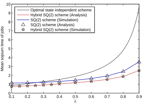
[image:15.612.183.424.79.255.2]Optimal state independent scheme Hybrid SQ(2) scheme (Analysis) SQ(2) scheme (Simulation) SQ(2) scheme (Analysis) Hybrid SQ(2) scheme (Simulation)
Fig. 1. Mean sojourn time jobs as a function ofλforC1= 2/3,C2= 4/3,N= 200andγ1=γ2= 1/2
their proportions is sufficient. Indeed, it is easy to see that choosing the sampling probabilities as:pi=PMγiCi j=1γjCj
for eachi∈ J givesΛas the stability region.
Such a sampling bias will not necessarily minimize the average delay.
IV. NUMERICAL RESULTS
In this section, we present simulation results to compare the different load balancing schemes considered in this
paper. The results also indicate the accuracy of the asymptotic analyses of the SQ(2) and the hybrid SQ(2) schemes
in predicting their performance in a finite system of servers. We set µ = 1 in all our simulations. We also plot
the simulation results for the SQ(5) scheme whose analysis and characterization is extremely complicated in the
heterogeneous case but can be shown to be superior to the SQ(2) case by coupling arguments. But as argued by
[5], [7] most of the gains are achieved (super-exponential decay of the tail distributions) by considering the SQ(2)
scheme - the focus of this paper.
We first set C1 = 4/3, C2 = 2/3, N = 200 and γ1 = γ2 = 12. Using conditions (1), (6) it is found that
Λ = Λ∞ = {0≤λ <1}. In Figure 1, we plot the mean sojourn time jobs in the system as a function of the
normalized arrival rate,λ, for the three schemes. It is observed from the plot that the SQ(2) scheme performs better
than Scheme 1 for higher values ofλand the hybrid SQ(2) scheme results in the least mean sojourn time of jobs
among all the three schemes.
The performance of the SQ(2) scheme may not always be better than that of Scheme 1. To demonstrate this fact
we choose a second set of parameter values as follows: C1 = 5/3, C2 = 1/3, N = 200, and γ1 = γ2 = 1/2.
Under this parameter setting, we haveΛ ={0≤λ <1} andΛ∞={0≤λ <2/3}. Therefore, in this setting, the
asymptotic stability region under the SQ(2) scheme is a strict subset of the stability region under Scheme 1 and
0.1 0.2 0.3 0.4 0.5 0.6 0.7 0.8 0.9 0
1 2 3 4 5 6 7 8 9
λ
Mean sojourn time of jobs
[image:16.612.189.421.80.254.2]Optimal state independent scheme Hybrid SQ(2) scheme (Simulation) SQ(2) Scheme (Simulation) SQ(2) Scheme (Analysis) Hybrid SQ(2) scheme (Analysis) SQ(5) Scheme
Fig. 2. Mean sojourn time jobs as a function ofλforC1= 1/3,C2= 5/3,N= 200, andγ1=γ2= 1/2
0.1 0.2 0.3 0.4 0.5 0.6 0.7 0.8 0.9 1
1.5 2 2.5 3 3.5 4 4.5
λ
Mean sojourn time of jobs under the SQ(2) scheme
N=200 Asymptotic N=100 N=50 N=10
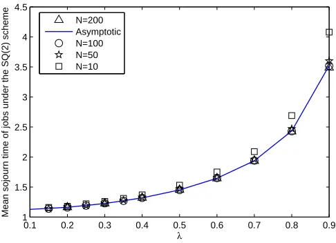
Fig. 3. Mean sojourn time jobs under the SQ(2) scheme as a function ofλfor different values ofN
schemes and the SQ(5) scheme. We see that the mean response time of jobs is lower in Scheme 1 than that in the
SQ(2) scheme. As in the previous setting, the hybrid SQ(2) scheme outperforms Scheme 1 and the SQ(2) scheme.
Furthermore, the SQ(5) scheme outperforms the SQ(2) scheme.
In Figure 3, we plot the mean sojourn time of jobs as a function ofλ for different values of the system size
N. The plots are obtained for the first parameter setting whereΛ = Λ∞. We observe a good match between the
asymptotic analysis and the simulation results forN= 50,100,200. The simulation results deviate from the analysis
forN= 10where the percentage of deviation is between 5-15%. This leads us to believe that the mean-field results
derived in this paper can be used to accurately predict the behavior of the schemes even for moderate number of
[image:16.612.181.424.315.491.2]The asymptotic insensitivity of the SQ(2) scheme. is numerically validated in Table I, where the the mean sojourn
time of jobs were obtained for the parameter setting C1 = 4/3,C2= 2/3,N = 200andγ1=γ2= 12. We chose
the following two distributions: i) constant, with distribution satisfyingF(x) = 0 for0≤x <1, andF(x) = 1,
otherwise. ii) power law, with distribution satisfying F(x) = 1−1/4x2 forx≥ 1
2 and F(x) = 0, otherwise. It
is seen that there is insignificant change in the mean sojourn time of jobs when the job length distribution type is
changed. The results, therefore, justify the asymptotic independence assumption stated in III-B.
TABLE I
INSENSITIVITY OF THESQ(2) SCHEME
λ Mean sojourn time
¯
T
Theoretical
Constant Simulation
Power Law Simulation 0.2 1.1614 1.1623 1.1620 0.3 1.2257 1.2257 1.2261 0.5 1.4547 1.4533 1.4550 0.7 1.9375 1.9377 1.9380 0.8 2.4265 2.4335 2.4330 0.9 3.5300 3.5204 3.5210
V. CONCLUSION
In this paper, we considered randomized load balancing schemes for large heterogeneous processor sharing
systems. It was shown that, as in the homogeneous case, the asymptotic stationary tail distribution of loads at each
server decreases doubly exponentially and is insensitive to the type of job length distribution under the SQ(2) scheme.
However, unlike the homogeneous case, in the heterogeneous case, the SQ(2) scheme has a smaller stability region
than the average capacity of the system. We have shown that the maximal stability region can be fully recovered
by using a scheme that combines the SQ(2) scheme with the state independent scheme and provides the best mean
sojourn time behaviour among all the schemes considered in the paper.
APPENDIX
A. Proof of Proposition 1
From condition (1.2) of [16] for any finite value of N, the system is stable under the SQ(2) scheme if the
following condition is satisfied:
max
B⊆S
X
i∈B C(i)
!−1
N λ µ
|B|
2
N
2
where S ={1,2, . . . , N} denotes the index set of servers, B ⊆ S is a subset of servers of size at least 2, and
C(k)∈ C denotes the capacity of thekth server in the system. Thus, forN =kN∗, the setΛk is given by
Λk =
λ >0 : X
i∈B C(i)
!−1
N λ µ |B| 2 N 2
<1 ∀ B ⊆ Sk
(39)
whereSk ={1,2, . . . , kN∗}. Clearly, for integers l andk, withl≥k, we haveSk⊆ Sl. Hence, if B ⊆ Sk, then
B ⊆ Sl. Therefore, from (39) it is clear thatλ∈Λl implies λ∈Λk. Consequently, for l≥k we haveΛk ⊇Λl.
Further, if we setB=S in (38) then we get (1). Hence, for allk∈N,Λ⊇Λk. This proves (4).
To prove (5), let us consider a finite value ofNand a setI ⊆ J. LetBI⊆ Sbe a subset of servers in which there
are ai (0< ai ≤N γi) servers of capacity Ci for each i∈ I. It can be easily checked that (
P
i∈Iai)(Pi∈Iai−1) P
i∈IaiCi
is an increasing function in each of the variablesai. Therefore, we have
X
i∈BI
C(i) !−1
N λ µ
|BI|
2 N 2 = λ µ P
i∈Iai Pi∈Iai−1
P
i∈IaiCi(N−1)
≤ λµ
P
i∈IN γi
P
i∈IN γi−1
P
i∈IN γiCi
(N−1)
≤ λ
µ
P
i∈IN γi Pi∈IN γi
P
i∈IN γiCi
(N)
= λ
µ
P
i∈Iγi
2
P
i∈IγiCi
The first equality follows from simplifying the expression on the L.H.S. The second inequality follows from the
first since we have N αN−1
−1 ≤
N α
N = α for α ≤ 1. Hence, λ ∈ Λ∞ implies
P
i∈BIC(i)
−1N λ µ
(|BI |
2 )
(N
2)
< 1. As
this is true for anyI ⊆ J and anyN, we have thatΛ∞⊆Λk for allk ∈N. Hence,Λ∞ ⊆ ∩∞k=1Λk. To prove
the reverse inclusion, considerλ∈ ∩∞
k=1Λk. ForI ⊆ J, consider a set B(IN) which contains all the N γi servers
of capacity Ci for eachi ∈ I. Since λ∈Λk for all k ∈N, we have limN→∞ Pi∈BIC(i)
−1N λ
µ
(|BI(N)|
2 )
(N
2) <1,
which is equivalent to the condition λµ (
P i∈Iγi)
2
(Pi∈IγiCi) <1. As this is true for all I ⊆ J, we have λ∈Λ∞. Hence, Λ∞=∩∞k=1Λk as required.
B. Proof of Proposition 2
i) Let Psatisfy the hypothesis of the proposition. Hence, from (12), we have that, for each l∈Z+ andj∈ J,
Pl(+1j) −Pl(+2j) =νj
Pl(j)−Pl(+1j)
M
X
i=1
γi
Pl(i)+Pl(+1i). (40)
Since by hypothesisPl(j)→0 as l→ ∞, adding the above equations forl≥k yields (13) upon simplification. ii) Equation (14) is a direct consequence of (13).
iii) From (14) we obtain γjP (j)
k+1
νj ≤
PM
j=1γjPk(j)
2
≤P˜k
2
, where P˜k = max1≤j≤MPk(j). Thus, we have
can choose k sufficiently large such thatδ <1. Hence, we have max1≤j≤MP
(j)
k+1
≤δP˜k. Similarly we have,
max1≤j≤MP
(j)
k+n
≤δ2n
−1P˜
k. This proves that the sequence
n
Pk(j), k∈Z+o decreases doubly exponentially for eachj.
C. Proof of Proposition 3
i) Defineθ(x) = [min(x,1)]+, where[z]+= max(0, z). Now, we consider the following modification of (9)-(12).
u(0) =g, (41)
˙
u(t) = ˜h(u(t)), (42)
where for1≤j≤M,
˜
h(0j)(u) = 0, (43)
˜
h(j)
n (u) =λ
h
θ(u(nj−)1)−θ(u(nj))
i
+
M
X
i=1
γi
h
θ(u(ni−)1) +θ(u(ni))
i
−µCj
h
θ(u(j)
n )−θ(u
(j)
n+1) i
+ (44)
for alln≥1. Note that the right hand side of (12) and (44) are equal ifu∈U¯M. Therefore, the two systems have the same solution inU¯M. Also if g∈U¯M, then any solution of the modified system remains within U¯M. This is because of the facts that if u(nj)(t) =un(j+1) (t) for somej, n,t, then h
(j)
n (u(t))≥0 and hn(j+1) (u(t))≤0, and if
u(nj)(t) = 0 for somej,n,t, thenh(nj)(u)≥0. Hence, to prove the uniqueness of solution of (9)-(12), we need to
show that the modified system (41)-(44) has a unique solution in(RZ+)M.
Using the norm defined in (16) and the facts that |x+−y+| ≤ |x−y| for any x, y ∈ R, |a1b1−a2b2| ≤
|a1−a2|+|b1−b2|for anya1, a2, b1, b2∈[0,1], and|θ(x)−θ(y)| ≤ |x−y| for anyx, y∈Rwe obtain
k˜h(u)k ≤K1 (45)
kh˜(u1)−˜h(u2)k ≤K2ku1−u2k, (46)
whereK1andK2 are constants defined asK1= 2λ+µ(max1≤j≤MCj)andK2= 8λ+ 2µ(max1≤j≤MCj). The
uniqueness follows from inequalities (45) and (46) by using Picard’s successive approximation technique sinceU¯M is complete under the norm defined in (16).
ii) For ease of exposition we provide a proof for theM = 2 case. The proof can be extended to anyM ≥2.
We note that if there exists P∈U¯M such that the sequencesnP(1) l , l∈Z+
o
and nPl(2), l∈Z+o satisfy the recursive relation (40) for alll∈Z+,j= 1,2, then it must be an equilibrium point of the system (9)-(12). Moreover,
ifPl(1), Pl(2) ↓0 as l→ ∞, then by Proposition 2.iii), such Pmust also lie in the spaceUM. We now proceed to
We construct the sequencesnPl(1)(α), l∈Z+o andnPl(2)(α), l∈Z+o as functions of the real variable α as follows:P0(1)(α) =P
(2)
0 (α) = 1,P (1)
1 (α) =α,P (2)
1 (α) = νγ22
1−γ1
ν1α
, and forl≥0andj = 1,2the following
recursive relationship holds
Pl(+2j)(α) =Pl(+1j)(α)−νj
Pl(j)(α)−Pl(+1j)(α)
2 X
i=1
γi
Pl(i)(α) +Pl(+1i)(α)
!
. (47)
Note that the above relation is same as (40). We show that there exists some value ofα, such that bothnPl(1)(α), l∈Z+o
andnPl(2)(α), l∈Z+oare non-negative, decreasing sequences (monotonicity will follow from non-negativity by virtue of (47)). It can be shown from the relations γ1
ν1P
(1)
1 (α) +γν22P
(2)
1 (α) = 1 and (47) that
2 X
j=1
γj
νj
Pl(+1j)(α) =
2 X
j=1
γjPl(j)(α)
2
forl≥0 (48)
From condition (6) and the construction above we see that for α ∈ max0,ν1
γ1
1−γ2
ν2
,min1,ν1
γ1
we
have1 =P0(j)(α)> P1(j)(α)>0 forj= 1,2. By using (47) forl = 2 andj= 1, we have that P2(1)(α)<0 for α= 0 andP2(1)(α)>0 forα= 1,ν1
γ1. Hence there must exist at least one root ofP
(1) 2 (α)in
0,min1,ν1
γ1
.
Let the maximum of these roots be r1. Therefore, if α ∈
maxr1,νγ11
1−γ2
ν2
,min1,ν1
γ1
then 1 =
P0(1)(α) > P1(1)(α)> P2(1)(α)>0. Similarly, for α=r1,νγ11
1−γ2
ν2
, we have P2(2)(α)>0 and for α= ν1
γ1 we have P2(2)(α) < 0. Therefore, there must exist a root of P
(2)
2 (α) in α ∈
maxr1,νγ11
1−γ2
ν2
,ν1
γ1
.
If we denote the minimum of these roots by r2, then for α ∈
maxr1,νγ11
1−γ2
ν2
,min (r2,1)
we get
1 = P0(j)(α)> P (j)
1 (α)> P (j)
2 (α) >0 forj = 1,2. Continuing in this way we can always get a range ofα∈
maxr2k+1,νγ11
1−γ2
ν2
,min (r2k+2,1)
such that 1 =P0(j)(α)> P (j)
1 (α)> P (j)
2 (α)> . . . > P (j)
k+2(α)>0
forj= 1,2. Hence, there exists a value ofαfor which the sequencesnPl(1)(α), l∈Z+oandnPl(2)(α), l∈Z+o
are non-negative, monotonically decreasing sequences in [0,1] starting at 1 satisfying (40). In other words there
existsαfor whichP(α) =nPl(j)(α), l∈Z+, j= 1,2ois inU¯M and is an equilibrium point of the system (9)-(12).
We now prove that for suchP(α),Pl(j)(α)→0as l→ ∞forj= 1,2.
We have seen that there exists a value ofαsuch that the sequencesnPl(1)(α), l∈Z+oandnPl(2)(α), l∈Z+o
are non-negative and monotonically decreasing sequences in [0,1]starting at1. Hence, by monotone convergence
theorem, both these sequences must converge in [0,1]. LetPl(1)(α) →ζ1 ∈[0,1]and Pl(2)(α)→ ζ2 ∈ [0,1] as
l→ ∞. Hence, by taking limit asl→ ∞on both sides of relation (48), we obtain
2 X
j=1
γj
νj
ζj =
2 X
j=1
γjζj
2
(49)
Expressing the above equation as a quadratic equationq(ζ1) inζ1 we see that that q(0) =γ1ζ2
γ2ζ2−ν12
<0
for 0 < ζ2 ≤ 1 since by (6) γ2ν2 < 1. Further, q(1) = γ22ζ22+
2γ1γ2−γν22
ζ2+
γ2 1−γν11
. By using the
stability condition (6) it can be easily shown that q(1)<0 if 0< ζ2≤1. Hence, either both roots or no roots of
conclude that there is no root ofq(ζ1) = 0in[0,1]if0< ζ2≤1. Hence,ζ2= 0. Forζ2= 0, the only solution of
q(ζ1) = 0 in[0,1]isζ1= 0. Therefore, we concludeζ1 =ζ2 = 0. Therefore, there exists a value ofα such that
Pl(1)(α), Pl(2)(α)↓0asl→ ∞. Thus, there existsαsuch thatP(α)∈ UM and is an equilibrium point of (9)-(12).
The uniqueness will follow from part (iii) of the proposition due to uniqueness of the limit.
iii) The proof is similar to the proof of Theorem 1.(iii) of [11] and hence is omitted to conserve space.
REFERENCES
[1] Y. Lu, Q. Xie, G. Kliot, A. Geller, J. R. Larus, and A. Greenberg, “Join-idle-queue: A novel load balancing algorithm for dynamically scalable web services,” Performance Evaluation, vol. 68, no. 11, pp. 1056–1071, 2011.
[2] E. Schurman and J. Brutlag, “The user and business impact on server delays, additional bytes and http chunking in web search,” in O’Reilly
Velocity Web Performance and Operations Conference, Jun. 2009.
[3] K. Salchow, “Load balancing 101: Nuts and bolts,” in White Paper, F5 Networks, Inc., 2007.
[4] V. Gupta, M. H. Balter, K. Sigman, and W. Whitt, “Analysis of join-the-shortest-queue routing for web server farms,” Performance
Evaluation, vol. 64, no. 9-12, pp. 1062–1081, 2007.
[5] N. D. Vvedenskaya, R. L. Dobrushin, and F. I. Karpelevich, “Queueing system with selection of the shortest of two queues: an asymptotic approach,” Problems of Information Transmission, vol. 32, no. 1, pp. 20–34, 1996.
[6] M. Mitzenmacher, “The power of two choices in randomized load balancing,” PhD Thesis, Berkeley, 1996.
[7] M. Mitzenmacher, “The power of two choices in randomized load balancing,” IEEE Transactions on Parallel and Distributed Systems, vol. 12, no. 10, pp. 1094–1104, 2001.
[8] C. Graham, “Chaoticity on path space for a queueing network with selection of shortest queue among several,” Journal of Applied
Probability, vol. 37, no. 1, pp. 198–211, 2000.
[9] M. Bramson, Y. Lu, and B. Prabhakar, “Asymptotic independence of queues under randomized load balancing,” Queueing Systems, vol. 71, no. 3, pp. 247–292, 2012.
[10] M. Bramson, Y. Lu, and B. Prabhakar, “Randomized load balancing with general service time distributions,” in Proceedings of ACM
SIGMETRICS, pp. 275–286, 2010.
[11] J. B. Martin and Y. M. Suhov, “Fast jackson networks,” Annals of Applied Probability, vol. 9, no. 3, pp. 854–870, 1999.
[12] E. Altman, U. Ayesta, and B. J. Prabhu, “Load balancing in processor sharing systems,” Telecommunication Systems, vol. 47, no. 1-2, pp. 35–48, 2008.
[13] S. N. Ethier and T. G. Kurtz, Markov Processes: Characterization and Convergence. John Wiley and Sons Ltd, 1985. [14] F. P. Kelly, Reversibility and Stochastic Networks. John Wiley and Sons Ltd, 1979.
[15] M. Aghajani and K. Ramanan, “Hydrodynamic limits of randomized load balancing networks.” preprint, Dept. of Applied Mathematics, Brown University, 2014.
[16] M. Bramson, “Stability of join the shortest queue networks,” Annals of Applied Probability, vol. 21, no. 4, pp. 1568–1625, 2011.
Arpan Mukhopadhyay received his Bachelors of Engineering (B.E) degree in Electronics and Telecommunication Engineering from Jadavpur
University, Culcutta, India in 2009, and his Master of Engineering (M.E) degree in Telecommunication from Indian Institute of Science, Bangalore, India in 2011.
Ravi Mazumdar (F’05) was born in April 1955 in Bangalore, India. He obtained the B.Tech. in Electrical Engineering from the Indian Institute of Technology, Bombay, India in 1977, the M.Sc. DIC in Control Systems from Imperial College, London, U.K. in 1978 and the Ph.D. in Systems Science from the University of California, Los Angeles, USA in 1983.
He is currently a University Research Chair Professor of Electrical and Computer Engineering at the University of Waterloo, Waterloo, Canada and an Adjunct Professor of ECE at Purdue University. He has served on the faculties of Columbia University (NY, USA) and INRS-Telecommunications (Montreal, Canada) . He held a Chair in Operational Research and Stochastic Systems in the Dept. of Mathematics at the University of Essex (Colchester, UK), and from 1999-2005 was Professor of ECE at Purdue University (West Lafayette, USA). He has held visiting positions and sabbatical leaves at UCLA, the University of Twente (Netherlands), the Indian Institute of Science (Bangalore), the Ecole Nationale Superieure des Telecommunications (Paris), INRIA (Paris) and the University of California, Berkeley.
He is a Fellow of the IEEE and the Royal Statistical Society. He is a member of the working groups WG6.3 and 7.1 of the IFIP and a member of SIAM and the IMS. He is a recipient of the IEEE INFOCOM 2006 Best Paper Award and was runner-up for the Best Paper at INFOCOM 1998,
0.1 0.2 0.3 0.4 0.5 0.6 0.7 0.8 0.9 0
1 2 3 4 5 6 7 8
λ
Mean sojourn time of jobs
Optimal state independent scheme Optimal SQ(2) scheme
0.1 0.2 0.3 0.4 0.5 0.6 0.7 0.8 0.9 0
1 2 3 4 5 6 7 8 9
λ
Mean sojourn time of jobs
Optimal state independent scheme Hybrid SQ(2) scheme (Analysis) SQ(2) scheme (Simulation) SQ(2) scheme (Analysis)