The value of relationships : evidence from a supply shock to Kenyan rose exports

http://wrap.warwick.ac.uk/

Macchiavello, Rocco and Morjariay, Ameet (2013) The value of relationships : evidence from a supply shock to Kenyan rose exports. Working Paper. Coventry, UK: University of Warwick, Department of Economics. (Warwick economics research papers series

(TWERPS)).

Permanent WRAP url:

http://wrap.warwick.ac.uk/59370

Copyright and reuse:

The Warwick Research Archive Portal (WRAP) makes this work of researchers of the University of Warwick available open access under the following conditions. Copyright © and all moral rights to the version of the paper presented here belong to the individual author(s) and/or other copyright owners. To the extent reasonable and practicable the material made available in WRAP has been checked for eligibility before being made available.

Copies of full items can be used for personal research or study, educational, or not-for-profit purposes without prior permission or charge. Provided that the authors, title and full bibliographic details are credited, a hyperlink and/or URL is given for the original metadata page and the content is not changed in any way.

A note on versions:

The version presented here is a working paper or pre-print that may be later published elsewhere. If a published version is known of, the above WRAP url will contain details on finding it.

The Value of Relationships:

Evidence from a Supply Shock to Kenyan Rose

Exports

Rocco Macchiavello and Ameet Morjaria

No 1032

WARWICK ECONOMIC RESEARCH PAPERS

The Value of Relationships: Evidence from a Supply

Shock to Kenyan Rose Exports

Rocco Macchiavello

Warwick, BREAD and CEPR

Ameet Morjaria World Bank

June 2013

Abstract

This paper provides evidence on the importance of reputation, intended as beliefs buyers hold about seller’s reliability, in the context of the Kenyan rose export sector. A model of reputation and relational contracting is developed and tested. We show that 1) the value of the relationship increases with the age of the relationship; 2) during an exogenous negative supply shock sellers prioritize relationships consistently with the predictions of the model; and 3) reliability at the time of the shock positively correlates with future survival and relationship value. Models exclusively focussing on enforcement or insurance considerations cannot account for the evidence.

Keywords: Relational Contracts, Reputation, Exports. JEL Codes: C73, D23, L14, O12.

1

Introduction

Imperfect contract enforcement is a pervasive feature of real-life commercial

transac-tions. In the absence of formal contract enforcement trading parties rely on informal

mechanisms to guarantee contractual performance (see, e.g., Johnson, McMillan and

Woodru¤ (2002), Greif (2005), Fafchamps (2006)). Among those mechanisms,

long-term relationships based on trust or reputation are perhaps the most widely studied

and have received substantial theoretical attention. The theoretical literature has

de-veloped a variety of models that capture salient features of real-life relationships, e.g.,

enforcement problems (see, e.g., MacLeod and Malcomsom (1989), Baker, Gibbons,

and Murphy (1994, 2002), Levin (2003)), insurance considerations (see, e.g., Thomas

and Worrall (1988)), or uncertainty over parties commitment to the relationship (see,

e.g., Ghosh and Ray (1996), Watson (1999), Halac (2012)). While these di¤erent

models share the common insight that future rents are necessary to deter short-term

opportunism, they also di¤er in important respects. Empirical evidence on informal

relationships between …rms, therefore, has the potential to identify which frictions are

most salient in a particular context. In turn, such knowledge can be bene…cial for

policy, particularly in a development context. Empirical progress in the area, however,

has been limited by the paucity of data on transactions between …rms in environments

with limited or no formal contract enforcement and challenges in measuring future

rents and beliefs.

This paper provides evidence on the importance of reputation, intended as beliefs

buyers hold about seller’s reliability, in the context of the Kenyan rose export sector. A

survey we conducted among exporters in Kenya reveals that relationships with foreign

buyers are not governed by written contracts enforceable in courts. The perishable

nature of roses makes it impractical to write and enforce contracts on supplier’s

reli-ability. Upon receiving the roses, the buyer could refuse payment and claim that the

roses did not arrive in the appropriate condition while the seller could always claim

otherwise. The resulting contractual imperfections, exacerbated by the international

nature of the transaction, imply that …rms rely on repeated transactions to assure

contractual performance.

The analysis takes advantage of three features of this setting. First, unlike

do-mestic sales, all export sales are administratively recorded by customs. We use six

years of transaction-level data of all exports of roses from Kenya, including the names

of domestic sellers and foreign buyers, as well as information on units traded, prices

a well-functioning spot market, the Dutch Auctions.1 If roses transacted in the rela-tionships can be traded on the auctions, incentive compatibility considerations imply

that the spot market price can be used to compute a lower bound to the future value

of the relationship. Third, the reaction of the relationships to a negative exogenous

supply shock induced by the post-election violence in January 2008 provides a unique

opportunity to test the predictions of the reputation model and distinguish it from

alternative models.2

We …rst present a model of the relationship between a rose producer (seller) and

a foreign buyer (buyer). The set up of the model matches qualitative features of the

market under consideration. A version of the model with no contract enforcement,

developed along the lines of the relational contracts literature, is analyzed …rst. The

incentive compatibility constraints of the model clarify how information on quantities

transacted, prices in the relationships and auction prices, which are all observable in

the data, can be used to compute lower bounds to the value of the relationship for

the buyer and the seller. The model is then extended to consider uncertainty over the

seller’s type and to examine how reputational forces in‡uence seller’s reaction to the

negative shock.

We then test the predictions of the model. Measures of the value of the future

rents in the relationship for the buyers and the sellers are computed. The estimated

relationships values correlate positively with the age and past amount of trade in the

relationship. The results, which hold controlling for relationship (which include seller,

buyer and cohort), time and selection e¤ects, are inconsistent with the pure limited

enforcement version of the model but support the version with reputational dynamics.

At the time of the violence, exporters located in the region directly a¤ected by the

violence could not satisfy commitments with all buyers. The violence was a large shock

and exporters had to chose which buyers to prioritize. We document an inverted-U

shaped relationship between the age of the relationship with the buyers and the

re-liability in supply at the time of the violence. The demonstrated rere-liability at the

time of the violence correlates with relationship’s survival and future values, but less

1_{The “Dutch”, or “clock”, auction is named after the ‡ower auctions in the Netherlands. In a} Dutch auction the auctioneer begins with a high asking price which is lowered until some participant is willing to accept, and pay, the auctioneer’s price. This type of auction is convenient when it is important to auction goods quickly, since a sale never requires more than one bid.

so in older relationships. Both facts are predicted by the reputation model and are

not consistent with other models, e.g., those that exclusively focus on enforcement or

insurance considerations. We discuss the policy implications of these …ndings,

par-ticularly from the point of view of export promotion in developing countries, in the

concluding section.

The …ndings and methodology of the paper contribute to the empirical literature on

relationships between …rms. McMillan and Woodru¤ (1999) and Banerjee and Du‡o

(2000) are closely related contributions that share with the current paper a developing

country setting.3 In an environment characterized by the absence of formal contract enforcement, McMillan and Woodru¤ (1999) …nd evidence consistent with long term

informal relationships facilitating trade credit. Banerjee and Du‡o (2000) infer the

importance of reputation by showing that a …rm’s age strongly correlates with

con-tractual forms in the Indian software industry. Both McMillan and Woodru¤ (1999)

and Banerjee and Du‡o (2000) rely on cross-sectional survey evidence and cannot

con-trol for unobserved …rm, or client, heterogeneity. In contrast, we exploit an exogenous

supply shock and rely on within relationship evidence to prove the existence, study

the source, and quantify the importance of the future rents necessary to enforce the

implicit contract. Antras and Foley (2012) and Macchiavello (2010) are two closely

related studies in an export context. Antras and Foley (2012) study the use of

prepay-ment to attenuate the risk of default by the importer. Using data from a U.S. based

exporter of frozen and refrigerated food products they …nd that prepayment is more

common at the beginning of a relationship and with importers located in countries

with a weaker institutional environment. Macchiavello (2010), instead, focuses on the

implications of learning about new suppliers in the context of Chilean wine exports.

In the context of domestic markets, particularly for credit and agricultural products,

Fafchamps (2000, 2004, 2006) has documented the importance of informal relationships

between …rms in Africa and elsewhere.4

The rest of the paper is organized as follows. Section 2 describes the industry,

its contractual practices, and the ethnic violence. Section 3 introduces the model

and derives testable predictions. Section 4 presents the empirical results. Section 5

provides a discussion of the …ndings. Sections 6 o¤ers some concluding remarks and

policy implications. Proofs, additional results and further information on the data are

relegated to an online Appendix.

2

Background

This section provides background information on the industry, its contractual

prac-tices and the ethnic violence. The section relies on information collected through a

representative survey of the Kenya ‡ower industry conducted by the authors through

face-to-face interviews in the summer of 2008.

2.1 The Kenya Flower Industry

Over the last decade, Kenya has become one of the largest exporters of ‡owers in the

world. The ‡ower industry, one of the largest foreign-currency earners for the Kenyan

economy, counts around one hundred established exporters located at various clusters

in the country. Roses, the focus of this study, account for about 80% of exports of

cut ‡owers from Kenya. Roses are a fragile and perishable commodity. To ensure

the supply of high-quality roses to distant markets, coordination along the supply

chain is crucial. Roses are hand-picked in the …eld, kept in cool storage rooms at a

constant temperature for grading, then packed, transported to Nairobi’s international

airport in refrigerated trucks owned by …rms, inspected and sent to overseas markets.

The industry is labor intensive and employs mostly low educated women in rural

areas. Workers receive training in harvesting, handling, grading, packing and acquire

skills which are di¢ cult to replace in the short-run. Because of both demand (e.g.

particular dates such as Valentines day and Mothers day) and supply factors (it is

4

costly to produce roses in Europe during winter), ‡oriculture is a seasonal business.

The business season begins in mid-August.

2.2 Contractual Practices

Roses are exported in two ways: they can be sold in the Netherlands at the Dutch

auctions or can be sold to direct buyers located in the Netherlands or elsewhere

(in-cluding Western Europe, Russia, Unites States, Japan and the Middle East). The

two marketing channels share the same logistic operations associated with exports,

but di¤er with respect to their contractual structure. The Dutch auctions are close

to the idealized Walrasian market described in textbooks. There are no contractual

obligations to deliver particular volumes or qualities of ‡owers at any particular date.

Upon arrival in the Netherlands, a clearing agent transports the ‡owers to the

auc-tions where they are inspected, graded and …nally put on the auction clock. Buyers

bid for the roses accordingly to the protocol of a standard descending price Dutch

auc-tion. The corresponding payment is immediately transferred from the buyer’s account

to the auction houses and then to the exporter, after deduction of a commission for

the auctions and the clearing agent. Apart from consolidating demand and supply

of roses in the market, the Dutch Auctions act as a platform that provides contract

enforcement between buyers and sellers located in di¤erent countries: they certify the

quality of the roses sold and enforce payments from buyers to sellers. It is common

practice in the industry to keep open accounts at the auctions houses even for those

…rms that sell their production almost exclusively through direct relationships. The

costs of maintaining an account are small, while the option value can be substantial.

Formal contract enforcement, in contrast, is missing in the direct relationships

between the ‡ower exporter and the foreign buyer, typically a wholesaler. The export

nature of the transaction and the high perishability of roses makes it impossible to

write and enforce contracts on supplier’s reliability. Upon receiving the roses, the buyer

could refuse payment and claim that the roses sent were not of the appropriate variety

and/or did not arrive in good condition. The seller could always claim otherwise.

Accordingly, exporters do not write complete contracts with foreign buyers.5

Exporters and foreign buyers negotiate a marketing plan at the beginning of the

5

season. With respect to volumes, the parties typically agree on some minimum volume

of orders year around to guarantee the seller a certain level of sales. Parties might,

however, agree to allow for a relatively large percentage (e.g., 20%) of orders to be

managed “ad hoc”. With respect to prices, most …rms negotiate constant prices with

their main buyer throughout the year but some have prices changing twice a year,

possibly through a catalogue or price list. Prices are not indexed on quality nor on

prices prevailing at the Dutch auctions.

Contracts do not specify exclusivity clauses. In particular, contracts do not require

…rms to sell all, or even a particular share, of their production to a buyer or to not sell

on the spot market. In principle, it would seem possible to write enforceable contracts

that prevent …rms from side-selling roses at the auctions. The ability to sell on the spot

market, however, gives producers ‡exibility to sell excess production as well as some

protection against buyers defaults and/or opportunism. Such contractual provisions

might not be desirable.

This paper takes the existence of direct relationships as given and does not explain

why relationships coexist along-side a spot-market.6 _{Beside lower freight and time} costs, a well-functioning relationship provide buyers and sellers with stability.

Buy-ers commitment to purchase pre-speci…ed quantities of roses throughout the season

allows sellers to better plan production. Buyers value reliability in supply of roses

often sourced from di¤erent regions to be combined into bouquets. Parties trade-o¤

these bene…ts with the costs of managing and nurturing direct relationships in an

environment lacking contract enforcement.

2.3 Electoral Violence

An intense episode of ethnic violence a¤ected several parts of Kenya following contested

presidential elections at the end of December 2007. The ethnic violence had two major

spikes lasting for a few days at the beginning and at the end of January 2008. The

regions in which rose producers are clustered were not all equally a¤ected. Only …rms

located in the Rift Valley and in the Western Provinces were directly a¤ected by the

violence (see Figure 1).7 The main consequence of the violence was that …rms located in the regions a¤ected by the violence found themselves lacking signi…cant numbers

6

Similar two-tier market structures have been documented in several markets in developing countries (see Fafchamps (2006) for a review). The coexistence of direct relationships alongside spot markets is also observed in several other contexts, such as perishable agricultural commodities, advertising and diamonds. We are grateful to Jon Levin for pointing this to us.

7

of their workers. Among the 74 …rms surveyed, 42 were located in regions that were

directly a¤ected by the violence. Table A1 shows that while …rms located in regions

not a¤ected by the violence did not report any signi…cant absence among workers (1%,

on average), …rms located in regions a¤ected by the violence reported an average of

50% of their labor force missing during the period of the violence. Furthermore, …rms

were unable to completely replace workers. On average, …rms in areas a¤ected by the

violence replaced around 5% of their missing workers with more than half of the …rms

replacing none. Many …rms paid higher over time wages to remaining workers in order

to minimize disruption in production.

With many workers missing, …rms su¤ered large reductions in total output. Figure

2 plots deseasonalized export volumes around the period of the violence for the two

separate groups of …rms. The Figure illustrates that the outbreak of the violence was

a large and negative shock to the quantity of roses exported by the …rms in the con‡ict

locations.

In the survey, we asked several questions about whether the violence had been

anticipated or not. Not a single …rm among the 74 producers interviewed reported

to have anticipated the shock (and to have adjusted production or sales plans

accord-ingly): the violence has been a large, unanticipated and short-run negative shock to

the production function of …rms.

2.4 Relationships Characteristics

Using the customs data, we build a dataset of relationships. Overall, we focus on the

period August 2004 to August 2009, i.e., …ve entire seasons. The violence happened

in January 2008, i.e., in the middle of the fourth season in the data, which runs from

August 2007 to August 2008.

We de…ne the baseline sample of relationships as those links between an exporter

and a foreign buyer that were active in the period immediately before the violence. A

relationship is active if the two parties transacted at least twenty times in the twenty

weeks before the eruption of the violence. The data show clear spikes in the distribution

of shipments across relationships at one, two, three, four and six shipments per week in

the reference period. The cuto¤ is chosen to distinguish between relationships versus

sporadic orders. Results are robust to alternative cuto¤s.

In total, this gives 189 relationships in the baseline sample. Panel A in Table 1

reports summary statistics for the relationships in the baseline sample. The average

age of the relationship in the sample, measured as the number of days from the …rst

shipment observed in the data, is 860 days, i.e., two years and a half. Immediately

before the violence, contracting parties in the average relationship had transacted with

each other 298 times.8

Exporters specialize in one marketing channel alone. The majority of exporters

either sells more than 90% of produce through direct relationships, or through the

auctions. As a result, among the one hundred established exporters, only …fty six

have at least one direct relationship with a foreign buyer in our baseline sample. On

average, therefore, exporters in the sample have three direct relationships (see Panel B

in Table 1). Similarly, there are seventy one buyers with at least a relationship in our

baseline. The average buyer, therefore, has about two and a half Kenyan suppliers.

Figures 3 and 4 document stylized facts that guide the formulation of the model.

Figure 3 shows that prices at the auctions are highly predictable. A regression of weekly

prices at the auction on week and season dummies explains 76% of the variation in prices in the three seasons preceding the violence period. Figure 4 shows that prices

in relationships are more stable than prices at the auctions.

3

Theory

This section introduces a work horse model of the relationship between a ‡ower

pro-ducer (seller) and a foreign buyer (buyer). The benchmark case with perfectly

en-forceable contracts is introduced …rst. The assumption of enen-forceable contracts is

then relaxed. The model predicts stationary dynamics which are inconsistent with the

empirical evidence. An extension with uncertainty about seller’s reliability is next

in-troduced. The extension matches the empirical evidence and is used to derive further

predictions on how sellers react to the violence. The section concludes with a summary

of testable implications.9

3.1 Set Up and First Best

Time is an in…nite sequence of periods t, t= 0;1; :::The buyer and the seller have an in…nite horizon and share a common discount factor <1:Periods alternate between

8

These averages are left-censored, since they are computed from August 2004 onward. Since our records begin in April 2004, we are able to distinguish relationships that were new in August 2004 from relationships that were active before. Among the 189 relationships in the baseline sample, 44% are classi…ed as censored, i.e., were already active before August 2004. This con…rms the …ndings of the survey, in which several respondents reported to have had relationships longer than a decade.

9

high seasonst= 0;2; :::and low seasonst= 1;3:::. Low season variables and parameters are denoted with a lower bar (e.g., x). Similarly, high season variables are denoted

with a upper bar (e.g., x).

In each period, the seller can producequnits of roses at costc(q) = cq₂2:The buyer’s payo¤s from sourcingqunits of roses from this particular seller isr(q) = ₂vq v_2jq q _j: The kink at q captures the buyer’s desire for reliability and, for simplicity, we assume

q =q =q .

There is also a market for roses where buyers and sellers can trade roses. The price

at which sellers can sell,pm_t ;oscillates betweenp_tm=pin high seasons andpm_t =p < p in low seasons:Letqmbe the quantity of roses sold on the market and mbe the seller’s optimal pro…ts when she does not sell roses to the buyer. The buyer can purchase roses

in the market at price pb_t = pm_t + ; with > 0 capturing additional transport and intermediation cost.

Contracts are negotiated at the beginning of high seasons. Parties agree on constant

prices for the high season and the subsequent low season. The buyer has the

ex-ante bargaining power and o¤ers contracts at the beginning of the high season. With

constant prices, a contract in periodt;then, is given by_Ct=

n

q_t; q

t+1; wt

o

:A contract

speci…es quantities to be delivered in the high seasontwhen the contract is negotiated,

q_t;in the following low season,q

t+1;and a unit price to be paid upon delivery of roses, wt;which is constant across seasons.10

We omit the period subscriptt when this doesn’t create confusion and assume:

Assumption 1: > v > p > cq > p= 0:

With perfectly enforceable contracts the buyer o¤ers a contract _C = q; q; w to maximize her pro…ts across two subsequent high and low season, i.e.,

(q; q; w) =r(q) wq+ r(q) wq (1)

subject to the seller participation constraint

wq+pqm c(q+qm) + wq+pqm c(q+qm) m+ m: (2)

The seller’s participation constraint takes into account her sales on the spot market:

for a given contract with the buyer;the seller setsqm and qm to maximize her pro…ts. 1 0

Proposition 1: The buyer o¤ ers C =nq ; q ;p+ (c₁₊(q )=q )o: The seller accepts and sets qm= p_c q and qm= 0.

The optimal contract displays i) lower seasonality in direct sales than in sales to

the spot market, and ii) price compression, i.e.,p < w < p:Both features are observed

in the data. In a relationship with perfect contract enforcement the optimal contract

is repeated forever.

3.2 Limited Enforcement

As revealed by interviews in the …eld, contracts enforcing the delivery of roses are not

available. This, potentially, generates two problems. First, the buyer might refuse to

pay the seller once the roses have been delivered. Second, given price compression, the

seller might fail to deliver the quantity of roses agreed with the buyer. Buyers and

sellers use relational contracts to overcome lack of enforcement.

A relational contract is a plan _CR = nq_t; q_t+1; wt

o1

t=0;2;::: that speci…es quantities

to be delivered, q_t and q_t+1;and unit prices, wt; for all future high and low seasons.

Parties agree to break-up the relationship and obtain their outside options forever

following any deviation. The outside option of the seller is to sell on the market

forever and the outside option of the buyer is normalized to zero. The buyer o¤ers the

relational contract to maximize the discounted value of future pro…ts

UR₀ =

1

X

t=0;2:::

t _(r(q

t) wtqt) + r q_t+1 wtq_t+1 (3)

subject to incentive compatibility constraints and the seller’s participation constraint.

Denote withU_tRand V_tRthe net present value of the payo¤s from the relationship at time t for the buyer and the seller respectively. Let U_tO and V_tO denote the net present value of the outside options. The buyer must prefer to pay the seller rather

than terminating the relationship, i.e.,

UR_t+1 UO_t+1 wt qt for allt= 0;2; ::: (4)

and

UR_t+2 UO_t+2 wt q_t+1 for all t= 0;2; ::: (5)

than optimally selling on the spot market, i.e.,

VR_t+1 VO_t+1 (p wt)qt for all for allt= 0;2; ::: (6)

and

VR_t+2 VO_t+2 wt q_t+1 +c(q_t+1) for all t= 0;2; ::: (7)

The relational contract_CRis chosen to maximize (3) subject to (4), (5), (6) and (7).11

Proposition 2: The optimal relational contract is such that qR_t =qR; qR_t+1 =qR

and wR_t =wR< pfor all t= 0;2; :::

The optimal relational contract is stationary. This is a well-known result (see, e.g.,

Abreu (1988) and Levin (2003)). The optimal relational contract also displays price

compression, i.e., wR < p: Price compression implies that (7) is never binding while constraint (6) always is. Constraint (4) can, therefore, be rewritten as

SR p qR (8)

whereSR=UR+VR VOis the value of the relationship. Lack of enforcement implies that the amount of roses traded is constrained by the future value of the relationship.

The incentive constraints (4) and (6), combined into (8) illustrate how data on auction

pricesp;relationship’s volumesqRand priceswRcan be used to estimate lower bounds to the value of the relationship to the buyer, the seller and as a whole. The quantity

b

S =pq provides a lower bound estimate of the value of the relationship. Sbis the sum of lower bound estimates of the value of the relationship for the seller Vb = (p w)q and for the buyer Ub = wq. The estimates S;b Vb and Ub are all directly observed in the data. Together with the quantity of roses traded when incentive constraints are

more likely to bind, Qb =qR;these are the main outcomes of interest in the empirical analysis. Future rents SR do not depend on current auction prices. A binding (8), therefore, implies an elasticity of qRwith respect to pequal to minus one.

3.3 Seller’s Hidden Types

Interviews in the …eld suggest that concerns over a seller’s reputation for reliability are

of paramount importance among buyers and sellers. First, delays and irregularity in

1 1

rose deliveries are costly to the buyer. Second, the sector has expanded rapidly and

many sellers lack a previous record of success in export markets.12

We follow the literature and model reputation introducing uncertainty over types.13 There are two types of sellers: reliable and unreliable. A reliable seller has a discount

factor equal to :An unreliable seller, instead, receives shocks which makes her

max-imize her instantaneous payo¤. The probability of the shock, ; is known to both

parties and is constant over time. At the beginning of the relationship, the buyer

believes that the seller is reliable with probability 0:

Contract terms, trade outcomes and relationship’s length are not observed by other

market participants. The buyer’s outside option is the value of returning to the market

to be matched with a new seller of uncertain type. We focus on pooling contracts and

equilibria in which the buyer terminates the relationship if the seller is revealed to be

unreliable.

The buyer faces a choice between supply assurance and learning. The buyer can

o¤er an initial pricewR

0 =pand ensure delivery in all periods regardless of the seller’s

type. A high price, however, is expensive and forces the buyer to trade relatively

low quantities of roses. Alternatively, the buyer can o¤er an initial price wR

0 < p: A

lower price relaxes the buyer’s incentive constraint but exposes the buyer to the risk of

non-delivery. As before, the buyer pays rents to the seller in the low season. Delivery

failure, therefore, doesn’t occur in the low season. However, a delivery failure still

occurs with probability (1 0) in the …rst high season:Delivery in the high season

(but not in the low season), therefore, conveys positive information about the seller’s

type. After periods of successful delivery the buyer holds beliefs ( )given by

( ) = 0

0+ (1 0) (1 )b =2c

; (9)

with 0( )>0and 00( )<0(for su¢ ciently large ):Conditional on delivery in the high season, the relationship is continued with positively updated beliefs about the

seller’s type.

Proposition 3: Suppose (8) is binding at the beginning of the relationship. There

exists such that for < the buyer experiments, i.e.: i) wR_t < p for all t and ii) 1 2_{Buyers must, of course, also develop a reputation for respecting contracts. Relative to suppliers,} which are all clustered in a handful of locations, buyers are scattered in several destination countries. Suppliers, therefore, can share information about cheating buyers more easily than buyers can share information about cheating suppliers. As a result, uncertainty over a seller’s reliability might be more relevant than uncertainty over buyer’s reliability.

1 3

qR_t+2 qR_t with a strict inequality for at least some initial t:

If is su¢ ciently low, the buyer prefers to risk non-delivery and experiment. Since

surplus increases in beliefs, ( );the optimal relational contract is non-stationary and the quantity sourced in the high season, alongside with relationship’s value, increases

with relationships’age.

3.4 The Violence

The violence hits the relationship in the middle of the high season (i.e., before the

unreliable type receives the shock to her discount rate). Consider a relationship of age

:The seller is supposed to deliver quantityqRat pricewR:Because of the violence, the seller can only deliver a share _{R 2}[0;1] ofqR:The share_R depends on unobservable e¤ort e eand on other random factors. The cost of e¤ort is (e):

Denote by _eeR _{and ee}U _{the buyer’s beliefs about the e¤ort exerted by the reliable}

and unreliable types respectively:In the equilibrium: 1) given buyer’s beliefs, a reliable

seller sets eR _{and an unreliable seller sets e}U _{to maximize expected payo¤, and 2)}

buyer’s beliefs are correct. As before, contracts, including adaptations of the relational

contract to information revealed at the time of the violence, are negotiated at the

beginning of the following high season.

We make the following assumptions:

Assumption 3:

1) 0( ) 0; 00( )>0, 0(0) = 0 and lim e!e

0_{(e) =1:}

2)_R is drawn from a Beta distribution f(_Rje) = Rae 1(1_B(e;e;aR)a(₎e e) 1 where aand e are positive constants such that e eand B( ) the appropriate Beta function:

The beta distribution is widely used to model the random behavior of percentages.

In our context, the beta distribution captures the intuition that higher e¤ort makes

high _R more likely while imposing su¢ cient regularity to derive comparative statics

results. In particular, the Beta distribution implies i) E[_Rje] =e_e; i.e., expected re-liability is linear in e¤ort, ii) monotone likelihood ratio, i.e., relatively higher _R is

a signal of relatively higher e¤ort, iii) higher e¤ort makes all states above a certain

threshold more likely and all states below less likely.

Proposition 4: Consider a relationship in which wR_{< p:In a separating}

doesn’t deliver any rose to the buyer and the relationship is terminated. Moreover, if

qR and Vb( ) = (p w )qR increase in ;the (expected) share of roses transacted at the time of the violence is increasing in relationship’s age if _e:

In a separating equilibrium in whicheR> eU, a high_Rconveys positive information about the seller’s type. A su¢ ciently low _R leads to beliefs that are too pessimistic

to sustain the relational contract. Anticipating this, the seller sells the available roses

on the spot market and the relationship ends. The last part of the proposition follows

from the trade-o¤ between the higher incentives provided by the desire to protect a

higher relationship’s valueVb against the standard diminished reputational incentives implied by su¢ ciently optimistic prior beliefs .

Conditional on the survival of the relationship, i.e., _{R R}e ; the relational con-tract is renegotiated at the beginning of the following high season. The new relational

contract is negotiated based on updated beliefs that depend on beliefs prior to the

violence, ( );equilibrium e¤ort levels, eRand eU;and observed reliability_R. These updated beliefs,e _R;_eeR;e_eU ;induce relationship valueS(e )in the high season fol-lowing the violence. The relationship valueS(e )is (weakly) increasing ine . Denoting

(_R) =f(_RjeeR)=f(_RjeeU), the updated beliefs are given by

e _R;_eeR;_eeU = (R)

(_R) + (1 ): (10)

The e¤ect of reliability _R on updated beliefs and, therefore, on relationship’s value

S(e );is positive for all relationship’s age and becomes negligible when prior beliefs are su¢ ciently optimistic:

3.5 Summary

The model provides the following three testable predictions:

Test 1: Consider outcomes _by_{2 f}Q;b S;b U ;b Vb_g:The pure limited enforcement model pre-dicts no correlation between the age of the relationship, ;and _by:The reputation model predicts a positive correlation between _by and an increasing and concave function of :

Test 3: The reputation model further predicts that: 1] Reliability at the time of the

violence, _Rb( );is an (initially) increasing and (possibly) inverted-U shape func-tion of an increasing and concave funcfunc-tion of ; 2] Conditional on age and survival, reliability at the time of the violence _Rb( ) positively correlates with future outcomes y_{b2 f}Q;b S;b U ;b Vb_g in the relationship. The correlation is weaker for older relationships.

4

Empirical Results

4.1 Incentive Constraints and the Value of Relationships

The incentive compatibility constraints (4) and (6), aggregated into (8), provide lower

bounds to the value of the relationship for the buyer, the seller and the relationship as

a whole. We denote these lower bounds asU; V and Srespectively. From an empirical

point of view, the appeal of the incentive constraints is thatqR_t; pand wR_t are directly observable in the data. The computation of the lower bounds U,V and S; therefore,

does not rely on information on the cost structure of the …rm, nor on expectations of

future trade between the parties, which are typically unobservable and/or di¢ cult to

estimate.

Recall that the model implies that only the maximum temptation to deviate has to

be considered to obtain an estimate of a lower bound to the value of the relationship.

For each relationship and season, therefore, we compute the lower bounds focusing on

the time in which the value of the roses on the market, qR_t p;is highest. In bringing the constraint to the data, we need to choose a temptation window, i.e., the length of

the period of time during which the temptation is computed. For simplicity, we focus

on temptation windows of a week.14 _{Denote calendar weeks with ! and let q}R i;t! be

the quantity traded in relationship i and pi;t! be auction prices in week ! of season

t: Using unit weight of roses transacted in relationshipi, it is possible to use auction

prices for large and small roses to index pi;t! by relationshipi: For each relationshipi

in seasont;de…ne week!_itas the one with the largest aggregate temptation to deviate, i.e.,

!_it= arg max ! q

R

i;t! pt! : (11)

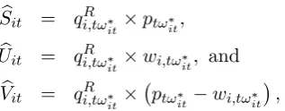
The lower bounds to the value of relationshipiin seasont, denoted bySbit;Ubit and

b

Vit;are given then by

b

Sit = qRi;t!_it pt!_it; (12)

b

Uit = qRi;t!_it wi;t!_it; and

b

Vit = qRi;t!_it pt!_it wi;t!_it ;

where wi;t! denotes the price paid in relationship i in week ! of season t: Together

withQbit=q_i;t!R

it;Sbit;UbitandVbitare the main outcomes in the empirical speci…cations.

The variation in the estimated values across time and relationships, therefore,

comes from di¤erent sources: i) the timing of the highest aggregate temptation, !_it;

ii) quantities transacted during the relevant window, q_i;t!R

it; iii) prices at the

auc-tion during the relevant window pt!_it; and iv) prices in the relationships during the

relevant window, wi;t!_it: Within seasons, prices in relationships are quite stable, i.e.,

wi;t! ' wi;t: Conditional on unit weight of roses, prices at the auctions do not vary

across relationships.

Figure 5 reports the distribution of weeks!_it in the sample used in Columns 1,3,5 and 7 of Table 2. The week of Valentine’s day is !_it in about 40% of relationships. Other prominent weeks are around Mother’s days, which typically fall in March (e.g.,

UK, Russia, Japan) or later in May (e.g., other European countries and U.S.)

depend-ing on the country. Since prices at the auctions are predictable (see Figure 3), the

estimated values are not driven by unexpectedly high prices.

For the 189 relationships in the baseline sample, Panel C in Table 1 shows that

the aggregate value of the relationshipSbin the season that preceded the violence was

578% of the average weekly revenues in the average relationship. The values for the buyer Ub and seller Vb respectively are387% and 191%of average weekly revenues.15

4.2 Test 1: Relationship’s Outcomes and Age

Figure 6 plots the distribution of the estimatedSbit (in logs) for three di¤erent samples

of relationships in the season before the violence: relationships in the baseline sample

that were active at the Valentine day peak of the season prior to the violence;

relation-ships in the baseline sample that were not active during the Valentine day peak of the

1 5

season prior to the violence; and relationships that were active during the Valentine

day peak of the season prior to the violence but that are not in the baseline sample

since they did not survive until the violence period. Figure 6 shows two patterns: i)

relationships that have survived have higher values than relationships that did not;ii)

young relationships had lower values than established relationships.

The latter observation, however, cannot be interpreted as evidence that the value

of a relationship increases with age. Mechanically, the estimated value of a relationship

that is too young to have gone through a seasonal peak is low. Table 2 presents

corre-lation patterns between recorre-lationship age and the four outcomes of interestQbit;Sbit;Ubit

and Vbit: Equation (9) in the theory section shows that beliefs about the seller’s type

are an increasing and (eventually) concave function of the past number of shipments in

which prices at the auctions were higher than prices in the relationship. Accordingly,

we measure age of the relationship as the log of the number of past shipments during

which prices at the auctions were higher than prices in the relationship and denote

this variable as log(N Tit): For all outcomes y 2 fQ; S; U; Vg odd numbered columns

in Table 2 report results that exploit cross-sectional variation in the season before the

violence, i.e.,

log (_byf b) = f + b+ log (N Tf b) +"f b; (13)

where _f and _b are exporter and buyer …xed e¤ects respectively and"f b is an error

term. The regression is estimated in the sample of relationships that were active in

the season before the violence.

From a cross-section it is not possible to disentangle age and cohort e¤ects. The

inclusion of buyer and seller …xed e¤ects controls for cohort e¤ects at the

contractual-party level, but does not control for relationship cohort e¤ects, i.e., the fact that more

valuable relationships might have started earlier. Even numbered columns in Table

2, therefore, present results from an alternative speci…cation that exploits the time

variation across seasons. This allows to include relationship …xed e¤ects that control

for time-invariant relationship characteristics, including cohort e¤ects. Normally, even

with panel data it is not possible to separately identify age, cohort and season e¤ects

since, given a cohort, age and seasons would be collinear. However, our measure of

the age of the relationship, log (N Tf b);is a non-linear function of calendar time and,

therefore, allows us to include season …xed e¤ects, i.e.,

where _{f b}are relationship …xed e¤ects, _tseason …xed e¤ects and"f btis an error term.

The selection e¤ect documented in Figure 6 could induce a spurious positive

correla-tion. The speci…cation is therefore estimated on a balanced sample of relationships

that where active in all three seasons prior to the violence.

Results in Table 2 indicate a strong, positive, correlation between relationship’s age

and outcomes. Regardless of whether cross-sectional or time variation are used, the

age of the relationship positively correlates with i) volumes traded at the time of the

highest temptation Qbit (columns 1 and 2),ii) the aggregate value of the relationship

b

Sit (columns 3 and 4), iii) the value of the relationship for the buyer Ubit (columns 5

and 6) and iv) for the sellerVbit (columns 7 and 8).16

4.3 Test 2: Binding Incentive Constraint

The results in Table 2 reject the predictions of the pure enforcement model. The results

are potentially consistent with the reputation model. The reputation model implies

the dynamics found in the data when the incentive constraint (8) is binding. Table 3

provides evidence suggesting that constraint (8) is binding in many relationships.

The logic for testing whether (8) is binding is as follows. In the model, the future

value of the relationship, Sbit; does not depend on current auction prices. If (8) is

binding, therefore, a small increase in prices at the auctions should lead to a

corre-sponding decrease in the quantity Qbit: Table 3 reports correlations between prices at

the auctions and relationship’s value Sbit (column 1) and quantities Qbit (column 2) in

the week of the highest temptation to deviate. In practice, relationship’s value might

depend on expectations of future prices at the auctions. Figure 3 shows that seasonal

variation in auction prices is highly predictable. Controlling for season and seasonality

…xed e¤ects, therefore, should account for parties expectations about future auction

prices. Seasonality …xed e¤ects are accounted for by including dummies for the week of

the season during which the highest temptation to deviate occurs. The combination of

season and seasonality e¤ects implies that variation in prices at the auctions captures

small unanticipated variation around the expected prices.

Table 3 shows that higher prices at the auctions lead to a proportional reduction in

1 6

The results in Table 2 are extremely robust to a variety of di¤erent assumptions and speci…cations. In particular: 1) outcomesQbit;Sbit;Ubit andVbitand age can be measured in levels, instead of logs; 2)

age can also be measured as the number of previous shipments, or the calendar time from the …rst shipment in the relationship; 3) relationships for which estimatedVbitare negative can also be included

(assigning them value of zero); 4) relationship controls, including week of maximum temptation to deviate !f b dummies, can be included; and 5) we do not …nd evidence of any di¤erence in results

quantity traded (column 2) and that, as a result, the aggregate value of roses traded

remains constant (column 1). The estimated elasticity between Qbitand auction prices

is equal to ( 0:884); which is very close (and not statistically di¤erent from) to the ( 1) implied by a binding (8). Increasing prices paid to the seller does not help relaxing the aggregate incentive constraint (8) since a reduction in the seller’s temptation to

deviate is compensated by an equal increase in the buyer’s temptation. Column (3)

shows that prices at the auctions do not lead to higher prices in the relationship.17 Taken together, the evidence is consistent with information from interviews suggesting

that parties often agree to allow for a percentage (e.g., 20%) of orders to be managed

“ad hoc” and avoid price renegotiations during the season.

4.4 Test 3: Predictions of the Reputation Model

Reliability at the Time of the Violence

This section provides further empirical tests of the predictions of the reputation

model by examining how relationships reacted to the violence. We exploit the

regu-larity of shipments within relationships to construct a counterfactual measure of the

volumes of roses that should have been exported in a particular relationship during

the time of the violence, had the violence not occurred. For each relationship in the

baseline sample, we separately estimate a model that predicts shipments of roses in a

particular day. The model includes shipments in the same day of the week the previous

week, total shipments in the previous week, week and season …xed e¤ects as regressors.

For each relationship, we obtain a predicted shipment of roses on a particular day. We

aggregate these predicted value at the week level. The model predicts more than 80%

of both in and out of sample variation in weekly shipments for the median relationship

in the sample.

Denote by yf b the observed shipments of roses in the relationship between …rm

f and buyer b during the week of the violence, and by y_bf b the predicted shipments

of roses in the same relationship, obtained using the observed shipments in the week

immediately before the violence and the coe¢ cients from the relationship speci…c model

1 7

described above. Reliability at the time of the violence is given by

b

Rf b=

yf b

b

yf b

: (15)

Table 4 shows that the violence reduced reliability _Rbf b. Table 4 reports results

from the regression

log_Rbf b= b+ ICf=1 + Zf b+ Xf+"f b; (16)

whereIC_f=1 is an indicator function that takes value equal to one if …rmf is located in the region a¤ected by the violence and zero otherwise;Xf is a vector of …rm controls,

Zf b is a vector of relationship controls, and b are buyer …xed e¤ects.

Relation-ship controls are age and the number of Relation-shipments, average price and volumes in the

twenty weeks preceding the violence. Seller controls are size (in hectares of land under

greenhouses), fair trade certi…cation, age of the …rm, membership in main business

association and ownership dummies (foreign, domestic Indian, indigenous Kenyan).

The reliability measure_Rbf b is a deviation from a relationships-speci…c counterfactual

that accounts for relationship-speci…c average and seasonal ‡uctuations in exports.

The controls included in speci…cation (16), then, allow the violence period to have

a¤ected export volumes in a particular relationship di¤erentially across buyers, sellers

and relationship characteristics.18

Table 4 shows that the violence reduced reliability. The Table reports results

using di¤erent empirical speci…cations that di¤er in the number of controls included.

In column 4, which controls for buyer …xed e¤ects as well as …rm and relationship

controls, reliability was almost20%lower, on average, in relationships of …rms located in the con‡ict region.19

Reliability and Relationship’s Age

Given the positive correlation between relationship age and value for the seller

found in Table 2, the reputation model predicts that sellers in older relationships have

stronger incentives to exert e¤ort during the violence and deliver roses to the buyers.

1 8_{The results from speci…cation (16), therefore, are equivalent to those of a regression of volumes of} exports y_ef b sat time in seasons;on relationship-speci…c seasonality and season …xed e¤ects, f b

and _{f bs}; in which the e¤ects of the violence are recovered from an interaction between a dummy for the period of the violence, v s;and a dummy for the con‡ict region,cf, after controlling for the

interactions betweenv sand seller, buyer and relationship characteristics.

1 9

The use of logs minimizes outliers. Results are robust to using the level of reliability:For instance, the speci…cation corresponding to column 4 yields a coe¢ cient of 0:316with associated p-value0:07:

On the other hand, in very old relationships, relatively little uncertainty might be left

regarding the seller’s type. In those cases, even low delivery would not lead to overly

pessimistic beliefs about the seller’s type. The model, therefore, predicts a (initially)

positive and, potentially, inverted-U relationship between reliability and age.

Table 5 reports results from the regression

log_Rbf b= b+ f + 1log (N Tf b) + 2[log (N Tf b)]2+ Zf b+"f b (17)

where bare buyer …xed e¤ects andZf bare relationship controls described above. This

speci…cation is very similar to equation (16), but note that it now includes …rm …xed

e¤ects _f: We are interested in comparing how …rms responded di¤erentially across relationships. Given that …rms in the violence region faced very di¤erent conditions,

we include …rm …xed e¤ects and estimate regression (17) separately on the sample of

…rms located in the two regions.

Columns 1 and 2 provide results from relationships in the con‡ict region. Column 1

shows that older relationships have higher reliability. Column 2 includes the measure

of age squared and …nds patterns consistent with an inverted-U shape relationship

between age and reliability. The estimated coe¢ cients give b₁=2b_{2 '} 5:35: This ratio implies approximately one third of relationships in the con‡ict region for which

higher age correlates with lower reliability. Columns 3 and 4 repeat the exercise on

the sample of relationships from the no-con‡ict region and fails to …nd any evidence

of a relationship between age and reliability.20;21

Reliability and Relationship’s Survival

The model predicts that reliability at the time of the violence correlates with

sub-sequent outcomes in the relationships. We focus on the period starting from the

beginning of the season following the violence, i.e., after mid August 2008. This is the

period in which buyers and sellers (re-)negotiate the relational contract for the new

season.

2 0

Results are robust to a number of alternative speci…cations. In particular: 1) when age is measured with the log of the number of past shipment b1 = 0:93 (p-value 0.001) and b2 = 0:08 (p-value

0.021) in the con‡ict region; 2) when the level of _Rbf b is used results give b1 = 0:86(p-value 0.007)

and b₂ = 0:07 (with p-value 0.141) in the con‡ict region; 3) a speci…cation pooling both regions …nds similar results, with lower precision depending on the set of interactions included. In all cases

b₁=2b_2'5in the con‡ict region while no statistically signi…cant pattern is found in the no-con‡ict region. Results are available upon request.

2 1

More relationships did not survive to the following season in the con‡ict region (16

out of 94, i.e., 17%) than in the no-con‡ict region (8 out of 95, i.e., 8.5%). The

di¤er-ence in survival rate is statistically signi…cant at the 5 percent level. Table 6 explores

the relationship between reliability, age and relationship survival in the two regions

separately. In the con‡ict region (columns 1 and 2) reliability positively correlates

with relationships’ survival. No such relationship is found in the no-con‡ict region

(columns 3 and 4).22Since relationship’s value and reliability increase with age (Table 2 and Table 5 respectively), Table 6 implies that the violence destroyed relatively less

valuable relationships in the con‡ict region.

Relationship Outcomes Conditional on Survival

Table 7 reports results on the four outcomes Qbit; Sbit;Ubit and Vbit in the season

following the violence. The model predicts that higher reliability correlates with

bet-ter outcomes and that the strength of these relationship should be smaller for older

relationships. For all outcomes y _{2 f}Q; S; U; V_g, the Table reports results from the

speci…cation

log (_byf b) = f+ b+ 1log Rbf b + 2log (N Tf b)+ 3log Rbf b log (N Tf b)+ Zf b+"f b;

(18)

where, as before, _f and b are seller and buyer …xed e¤ects,logN Tf b is the preferred

measure of age before the violence, Rbf b is reliability at the time of the violence, Zf b

are relationship controls, and"f bis an error term. All independent variables, including

controls, measure relationship characteristics prior to the violence. The model predicts

1>0; 2>0and 3 <0:

Panel A in Table 7 considers the con‡ict region. For all four outcomes, results

indicate that higher reliability correlates with higher future outcomes in the

relation-ship, i.e., ₁ >0:Similarly, age at the time of the violence, measured by log (N Tf b);

positively correlates with outcomes Qb, Sb and Ub (though not Vb):The interaction be-tween age and reliability at the time of the violence is always negative and statistically

signi…cant, i.e., ₃ <0. Consistently with the predictions of the model, reliability at the time of the violence translated into better outcomes in younger relationships. For

all four outcomes, the Panel B fails to …nd any systematic pattern in the no con‡ict

region.23

4.5 E¤ort at the Time of the Violence

Tables A2 and A3 in the Appendix provide evidence that …rms exerted e¤ort during

the violence, as assumed in the model. Two margins of e¤ort are considered.

Fig-ure A1 in the Appendix shows that at the time of the violence prices in most direct

relationships were lower than prices on the spot market. Table A2 in the Appendix

shows that, despite higher prices at the auctions, export volumes to the spot market

dropped signi…cantly more than export volumes to direct buyers. This di¤erential

re-sponse holds controlling for seller …xed e¤ects, i.e., comparing sales to the two channels

within the same …rm. Table A3 in the Appendix shows that …rms that specialize in

selling to direct buyers retained higher percentages of their workers during the

vio-lence.24 _{Firms could retain workers by, e.g., setting up camps on or around the farm} for workers threatened by the violence and paying higher wages to compensate over

time for workers that were still working on the farm. The correlation holds controlling

for characteristics of the …rm’s labor force (education, gender, ethnicity, contract type

and housing programs), as well as …rm characteristics (ownership type, certi…cations

and land size). In sum, we …nd evidence that …rms exerted e¤orts along at least two

margins to respond to the violence.

5

Discussion

The evidence strongly supports the predictions of the reputation model: i) relationship

dynamics are non-stationary (Test 1),ii) the aggregate incentive constraint (8) appears

to be binding in many relationships (Test 2) and iii) the reaction to the violence are

consistent with further predictions of the reputation model (Test 3), e.g., the

non-linear relationship between age and reliability and the long-run e¤ects of reliability.

Before concluding, several points are worth discussing. We …rst consider the role of

unobserved rose characteristics and then discuss some of the key assumptions of the

model and how the evidence relates to alternative theoretical models.

2 3

Results in Table 7 are qualitatively similar in a number of alternative speci…cations. In particular, 1) the use of reliability in level (instead of log); 2) a pooled regression gives similar results with lower statistical signi…cance on outcomes Qb and Sb; 3) results are stronger when using levels of outcome variables. Results are available upon request.

5.1 Unobserved Rose Characteristics

The value of a rose mainly depends oni) its size, which we can proxy with unit weights

reported in the customs data, andii) its variety which, unfortunately, is not reported.

Unobserved characteristics of roses present two main concerns for our results. A …rst

concern regards the seller’s incentive constraint (6) and its empirical implementation

in (12). To estimate the lower bound to the value of the relationship we assumed

that the roses can be sold at the auctions. A violation of the assumption introduces

measurement error. The auctions are an extremely liquid market in which hundreds of

rose varieties are traded each day. Conversations with practitioners suggest that the

assumption is likely to be valid in most cases. Still, it is possible that for some

rela-tionships the assumption is violated at the time of the highest temptation to deviate.

Three aspects of the empirical results are somewhat reassuring regarding the

impor-tance of this source of measurement error. First, Table A4 in the Appendix shows

that, within …rms, there is no di¤erence in the average and standard deviation of unit

weights sold to direct buyers and to the auctions. Second, the predictions of the model

hold for two outcome variables,Qband U ;b that do not directly depend on prices at the auctions. Third, the evidence of a binding incentive constraint (8) in Table 3 suggests

that side-selling to the auction is the relevant deviation in most relationships.

A second concern is that …rms might export to di¤erent buyers varieties of roses

that are di¤erentially a¤ected by the violence (e.g., more labour intensive or perishable

varieties). If those rose characteristics correlate with the age of the relationship, the

results in Table 2 might be biased. Table A4 shows that average and standard deviation

of unit weights do not correlate with the age of the relationship. Further (unreported)

results show that average and standard deviation of unit weights do not change with

season and at the time of the violence within relationships. To the extent that data

allow, we do not …nd evidence that unobserved rose characteristics pose a threat to

our results.

5.2 Assumptions in the Model

Motivated by interviews in the …eld, we assumed that contracts are negotiated at

the beginning of the high season and that prices are constant across seasons. The

complexity associated with indexing contracts on weekly auction prices, the inability

of sellers and courts to observe the quality of roses delivered and a desire to smooth

abstract from these forces and take constant prices as a fact of commercial life in our

environment. If prices varied across seasons, the qualitative insights of the benchmark

and pure enforcement model would be una¤ected. The analysis of the model with

types, however, would require a di¤erent formulation of types and would become more

involved.

A second assumption is that outside options do not change over time. The

assump-tion is justi…ed by the fact that outside opassump-tions are likely to be funcassump-tions of seller’s

speci…c, rather than relationship’s speci…c, variables that evolve over time. The

em-pirical analysis controls for seller’s …xed e¤ects, e¤ectively comparing relationships

holding constant seller’s speci…c factors that could determine outside options.

We have focused our attention on pooling contracts. In models with dynamic

adverse selection it is possible, but potentially very costly, to screen types (see, e.g.,

La¤ont and Tirole (1988)). In our model, both types receive the same pay-o¤ which

is equivalent to their outside option. Screening, therefore, would require paying future

rents to the reliable type. The buyer’s incentive constraint, however, places limits

on future payments to the seller potentially limiting the availability of separating

contracts.

We have assumed that, following the violence, contracts are renegotiated at the

beginning of the following high season. The assumption simpli…es the de…nition of

the Bayesian equilibrium following the violence and the derivation of the results in

Proposition 4. The unforeseen nature of the shock, the distance between buyers and

sellers and the need for a prompt response make the assumption appealing from an

empirical point of view as well.

5.3 Informal Insurance

Insurance considerations could also be important determinants of the value of

rela-tionships in this context.25 Informal insurance models also predict non-stationary outcomes: past realizations of shocks in‡uence future continuation values. Because

past realization of shocks are unobservable it is di¢ cult to reject informal insurance

models. The results, however, suggest that insurance considerations are unlikely to

be driving how relationships reacted to the violence. First, insurance models predict

that relationships with higher promised value should give more slack to the seller. The

evidence suggests the opposite is true: older, and more valuable, relationships tend to

2 5

have higher reliability. Second, insurance considerations imply the use of both current

transfers and future values to provide incentives. In contrast, Figure A2 in the

Appen-dix shows that the distribution of prices at the time of the violence is very similar to

its counterpart in the twenty weeks before the violence. Prices were not renegotiated

upward at the time of the violence.

5.4 Alternative Modeling Assumptions

Levin (2003) extended the relational contracts literature (see, e.g., MacLeod and

Mal-comson (1989), Baker et al. (1994, 2002)) to the case of moral hazard and adverse

selection with i.i.d. types over time. Under both scenarios, provided that i) parties

are risk-neutral and have access to monetary transfers, and ii) the buyer’s actions are

perfectly observable; the (constrained) optimal relational contract is stationary. The

evidence, therefore, rejects extensions of the baseline model entirely based on this type

of asymmetric information.

Other modeling assumptions, however, imply non-stationary outcomes without

as-suming learning. When there is moral hazard and the buyer privately observes the

quality of the roses delivered stationary contracts are no longer optimal. Levin (2003)

and Fuchs (2007), however, show that the optimal contract is a termination contract

in which trade between parties continues in a stationary fashion provided performance

is above a certain threshold during a certain period of time. If performance falls below

the threshold, the relationship ends. The evidence is, therefore, also inconsistent with

this extension of the model.

Halac (2012) and Yang (2012) also study relational contract models with types. In

a model with binary e¤ort and output, Yang (2012) assumes that agents have di¤erent

productivity and obtains non-stationary outcomes. Halac (2012), instead, assumes

that either party has private information about her outside option and also obtains

non-stationary outcomes. In the special case in which the buyer has the bargaining

power and the seller has private information, however, the model predicts stationary

outcomes.26

6

Conclusion

Imperfect contract enforcement is a pervasive feature of real-life commercial

trans-actions. In the absence of formal contract enforcement trading parties rely on the

future rents associated with long term relationships to deter short-term opportunism

and facilitate trade. Empirical evidence on the structure of informal arrangements in

supply relationships between …rms has the potential to identify salient microeconomic

frictions in speci…c contexts and inform policy, particularly in a development context.

This paper presents an empirical study of supply relationships in the Kenya rose

ex-port sector, a context particularly well-suited to study informal relationships between

…rms.

We …nd evidence consistent with models in which sellers value acquiring and

main-taining a reputation for reliability. From a policy perspective, it is important to know

whether learning and reputation are important determinants of …rms’ success in

ex-port markets. Firms might have to operate at initial losses in order to acquire a good

reputation. Furthermore, if reputation is an important determinant of contractual

outcomes, prior beliefs about sellers a¤ect buyers willingness to trade, at least for a

while. This generates externalities across sellers and over time, justifying commonly

observed institutions such as certi…cations, business associations and subsidies to joint

marketing activities.

References

[1] Abreu, D. (1988) “On the Theory of In…nitely Repeated Games with Discounting”,

Econometrica, November 56(6), pp. 383-96.

[2] Andrabi, T., M. Ghatak and A. Kwhaja (2006) “Subcontractors for Tractors:

Theory and Evidence on Flexible Specialization, Supplier Selection, and

Con-tracting”, Journal of Development Economics, April 79 (2): 273-302.

[3] Antras, P. and F. Foley (2012) “Poultry in Motion: a Study of International Trade

Finance Practices”, mimeo Harvard

[4] Araujo, L. and E. Ornelas (2010) “Trust-based Trade”, mimeo LSE

[5] Baker, G., R. Gibbons and K. Murphy (1994) “Subjective Performance Measures

in Optimal Incentives Contracts”, Quarterly Journal of Economics, 109(4), pp.