Reduced order modelling of parameter dependent linear and nonlinear dynamic PDE models

(1)

warwick.ac.uk/lib-publications

Original citation:

Shah, A. A., Xing, W. W. and Triantafyllidis, V.. (2017) Reduced order modelling of parameter

dependent linear and nonlinear dynamic PDE models. Proceedings of the Royal Society A:

Mathematical, Physical and Engineering Sciences, 473 (2200). 20160809.

Permanent WRAP URL:

http://wrap.warwick.ac.uk/92604

Copyright and reuse:

The Warwick Research Archive Portal (WRAP) makes this work of researchers of the

University of Warwick available open access under the following conditions.

This article is made available under the Creative Commons Attribution 4.0 International

license (CC BY 4.0) and may be reused according to the conditions of the license. For more

details see:

http://creativecommons.org/licenses/by/4.0/

A note on versions:

The version presented in WRAP is the published version, or, version of record, and may be

cited as it appears here.

(2)

rspa.royalsocietypublishing.org

Research

Article submitted to journal

Subject Areas:

Computer modelling and simulation,

Computational mathematics,

Differential equations

Keywords:

Parameter-dependent partial

differential equations, proper

orthogonal decomposition, Gaussian

process model, manifold learning,

nonlinear systems

Author for correspondence:

A.A. Shah

e-mail: [email protected]

Reduced order modelling of

parameter dependent linear

and nonlinear dynamic PDE

models

A.A. Shah

1

, W.W. Xing

1

, V. Triantafyllidis

1

1_{School of Engineering, University of Warwick,}

Coventry CV4 7AL, UK

In this paper we develop reduced-order models (ROMs) for dynamic, parameter-dependent, linear

and nonlinear partial differential equations using proper orthogonal decomposition (POD). The main

challenges are to accurately and efficiently approximate the POD bases for new parameter values and, in

the case of nonlinear problems, to efficiently handle the nonlinear terms. We use a Bayesian nonlinear

regression approach to learn the snapshots of the solutions and the nonlinearities for new parameter

values. Computational efficiency is ensured by using manifold learning to perform the emulation in a

low-dimensional space. The accuracy of the method is demonstrated on a linear and a nonlinear example,

with comparisons to a global basis approach.

1. Introduction

Computational modelling is an indispensable tool for analysis, design, optimization and control. For

applications that require a high number of model evaluations at different inputs (e.g., uncertainty analysis

and inverse parameter estimation) the computational expense of a computer model is often prohibitive. In

such cases, the original computer model can be replaced with a surrogate model (or emulator) [1]. The simplest

approach to surrogate modelling consists of simplifying the mathematical model or numerical formulation, e.g.,

by assuming spatial homogeneity or using coarse grids.

c

The Authors. Published by the Royal Society under the terms of the Creative Commons Attribution License http://creativecommons.org/licenses/

by/4.0/, which permits unrestricted use, provided the original author and

(3)

2

rspa.ro

y

alsocietypub

lishing.org

Proc

R

Soc

A

0000000

..

The other two main approaches are based on: (i) supervised machine learning methods to learn the model input-output relationship (so called data-driven models); or (ii) Galerkin projection

schemes, to yield reduced order models(ROMs). The projecting basis in ROMs can be obtained through balanced truncation, Krylov subspaces or proper orthogonal decomposition (POD) (for

a recent survey we refer the reader to [5]). For partial differential equation (PDE) models, the Galerkin projection can be performed on the original equations (strong or a weak form) or on

the spatially discretized system. The final form is an algebraic system for steady problems or an ordinary differential equation (ODE) system in time for dynamical problems.

The most widely used technique for PDE systems is POD [2–4], in which the approximating subspace is obtained from solutions (called snapshots) generated by the discretized full-order

model (FOM) at selected time instances. Application of POD to dynamic, nonlinear parameterized PDEs presents a number of challenges: (i) constructing a basis that is valid across parameter

space; (ii) dealing with high-dimensional parameter spaces; (iii) using data parsimoniously; (iv)

efficiently computing the reduced-order system matrices and reduced-order nonlinearities in the state variable during use of the surrogate, i.e., the so calledonlinephase (we may also mention the

development of stable POD schemes to overcome instabilities in the original formulations). There are several approaches to incorporating parametric dependence: (a) to use a global

basis (meaning across parameter space); (b) interpolation of local bases (meaning for particular parameter values); and (c) interpolation of local system matrices. For linear time-invariant (LTI)

systems, the system matrices often take the form of affine combinations of constant matrices with parameter-dependent coefficients. In such cases the reduced-order system is quickly and easily

assembled for a new parameter value [6,7]. Affine forms can also be realized by using a Taylor series expansion [8] or an empirical interpolation strategy [9]. Global basis methods extract a

single basis from multiple local snapshot matrices [6,10,11]. Obvious drawbacks are the violation of POD optimality and the growth in the size of the global matrix with the number of samples.

There are, however, efficient sampling strategies for constructing global bases, such as the greedy approach of [6] or by using a local sensitivity analysis [12].

An alternative approach is interpolation of local bases or local reduced-model matrices. Lieuet al.[13] used the principal angles between two POD bases, pertaining to different Mach numbers,

to linearly interpolate a local basis for intermediate Mach numbers in a linearized fluid-structure ROM model. This method is restricted to single-parameter systems and small parameter changes.

Amsallem and Farhat considered local bases as members of a Grassmann manifold, the set of all subspaces (of a chosen low dimension) of the state space [14]. The local bases are mapped to a

tangent space of the Grassman manifold using a logarithmic map and Lagrange interpolation is performed in the tangent space. An inverse exponential map provides the required local bases.

Interpolation methods can also be used to approximate the reduced-order system matrices, in order to circumvent the problem of computing these matrices for each new parameter value.

Degroote et al. [11] proposed two methods: element-wise direct spline interpolation of the reduced-order matrices or spline interpolation of the matrices in a tangent space of a Riemannian

manifold on which the matrices are assumed to lie (a similar method was proposed in [15]). When

(4)

3

rspa.ro

y

alsocietypub

lishing.org

Proc

R

Soc

A

0000000

..

meaning from one local basis to another. Thus a congruency transformation to a common basis is required before direct interpolation [16] or interpolation in a tangent space [17].

Liebermanet al.used a greedy algorithm to construct projections for both the state variable and the parameters simultaneously, minimizing a measure of the error between the ROM and FOM

outputs at each iteration [18] (different error measures were considered in [19]). Hayet al. [20] used sensitivities (derivatives) of the POD basis with respect to (w.r.t.) the parameters to either

linearly extrapolate the POD basis for a new parameter value or to expand the POD basis by augmenting it with the corresponding sensitivities. The growth in the basis dimension with the

number of parameters is a limitation of this approach.

The computational cost of evaluating a strong (high-order polynomial or non-polynomial)

nonlinearity in the state variable in a ROM depends on the dimension of the original state space. Linearisation methods [21, 22] are only applicable to weak nonlinearities or confined regions

of state space. Moreover, the computational cost grows exponentially with the order of the

approximating expansion. Recently, a number ofhyper-reductionmethods have been developed to overcome the limitations of linearization approaches (see also the tensorial POD approach

recently developed in [25]). An early method was developed by Astrid et al. [23], based on selecting a subset of the FOM equations corresponding to heuristically chosen spatial grid points,

followed by a Galerkin projection of the resulting reduced system onto the POD basis.

The empirical interpolation method interpolates the nonlinear function at selected spatial

locations using an empirically derived basis, and is applied directly to the governing PDE [7], while the discrete empirical interpolation method (DEIM), is applicable to general ODE or

algebraic systems arising from a spatial discretization [24]. Both methods construct a subspace for the approximation of the nonlinear term and use a greedy algorithm to select interpolation

points. An extension of DEIM [26] generates several local subspacesvia clustering and uses classification in the online phase to select one of the subspaces. These approaches can also be

used for approximating (vectorized) non-affine system matrices [5]. The Gauss-Newton with approximated tensors (GNAT) method operates at the fully discrete level in space and time,

and is based on satisfying consistency and discrete-optimality conditions by solving a residual-minimization problem [27]. This leads to a Petrov-Galerkin (rather than Galerkin) problem with

a test basis that depends on the residual derivatives w.r.t. the state variable.

In this paper we introduce an extension of POD for dynamic, parameterized, linear and

nonlinear PDEs. The method we develop involves a computationally efficient approximation of the POD basis and the nonlinearity for new parameter values. It can be used in conjunction with

many of the methods described above, e.g., greedy sampling and methods for approximating non-affine system matrices. In order to avoid inconsistencies and to reduce the loss of information

in the construction of new bases, we take the approach of approximating the snapshots rather than the bases or system matrices directly. The snapshots, however, lie in high-dimensional spaces

so that direct approximations are computationally unfeasible. We overcome this issue by using manifold learning techniques [28] to map the snapshots to a low-dimensional feature space. We

then use Gaussian process emulation (GPE) to infer values of the mapped snapshots for new

parameter values, followed by an inverse map to obtain the snapshots in physical space. For nonlinear problems, we extend DEIM by using the same emulation approach to approximate

(5)

4

rspa.ro

y

alsocietypub

lishing.org

Proc

R

Soc

A

0000000

..

In the next section, we outline the procedures for generating ROMs and POD bases. We provide brief details of the DEIM and explain the issues associated with parameterized and/or

nonlinear problems. In Section3, we present the snapshot emulation strategy and summarize our approach to linear and nonlinear parameterized problems. In section4we present one linear and

one nonlinear example, comparing the results to a global basis approach.

2. ROMs for parameterized dynamic PDEs using POD

(a) Problem definition and Galerkin projection

Letx= (x1, . . . , xL)denote a point in a bounded, regular domainD ⊂RL(L= 1,2,3), lett∈[0, T] denote time and letξξξ∈ X ⊂Rldenote a vector of parameters. For the purposes of illustration,

consider a parameterized, parabolic PDE for a dependent variableu(x, t;ξξξ): ∂tu+L(ξξξ)u+N(ξξξ)u=g(x;ξξξ) (x, t)∈ D ×(0, T]

u(x,0;ξξξ) =u0(x;ξξξ) x∈ D

(2.1)

augmented by linear boundary conditions. Here,L(ξξξ)andN(ξξξ)are parameter dependent linear and nonlinear partial differential operators, respectively. The dependence on the parameters can

be through the operators, the source termg(x;ξξξ)or the initial/boundary conditions.

Let H be a separable Hilbert space with inner product (·,·)H and induced norm || · ||H,

e.g.,L2(D), the space of square integrable equivalence classes of functions with inner product

(v, v0)L2₍_D₎= R

Dv(x)v 0

(x)dx. From hereon, we drop the subscript in the notation for the inner product and norm inL2(D). It is assumed that for eachξξξ,u∈L2(0, T;H), i.e.,t7→u(·, t;ξξξ)is a Lebesgue measurable map from(0, T)toHwith finite norm||u||L2_(0,T;_H₎:=

RT

0 ||u(·, t;ξξξ)||Hdt. Thenu(·, t;ξξξ)∈ Hfor eacht∈(0, T). A spatial discretization of (2.1) leads to a system of ODEs:

˙

u(t;ξξξ) =A(ξξξ)u(t;ξξξ) +f(u(t;ξξξ);ξξξ), u(0;ξξξ) =u0(ξξξ) (2.2) for a discrete state variableu(t;ξξξ) = (u1(t;ξξξ), . . . , ud(t;ξξξ))T, which we call thesolution vector.d is the number of degrees of freedom, e.g., the number of grid points in a finite difference (FD)

approximation, the number of cells in a cell-centred finite volume (FV) approximation or the number of nodes (basis functions) in a finite-element (FE) approximation. The matrixA(ξξξ)∈Rd×d

arises from the linear termL(ξξξ)uandf(u(t;ξξξ);ξξξ)∈Rdarises from a combination ofN(ξξξ)u,g(x;ξξξ)

and possibly the boundary conditions. The latter is nonlinear forN(ξξξ)u6≡0.

The precise relationship betweenu(t;ξξξ)andu(x, t;ξξξ), the forms ofA(ξξξ)andf(u;ξξξ), and the incorporation of boundary conditions depend on the method used. For a FD approximation,

problem (2.1) is solved directly and the boundary conditions are incorporated inf(u;ξξξ). In a FE approximation a weak form is solved with test functions inHor a dense subspaceVofH, with

boundary conditions incorporated infand/or the definition ofH. The form ofA(ξξξ)is determined by the dependence ofL(ξξξ)onξξξ. The simplest case is an affine form:A(ξξξ) =P

ici(ξξξ)Ai, where the functionsci(ξξξ)are known and the matricesAiare constant.

(6)

5

rspa.ro

y

alsocietypub

lishing.org

Proc

R

Soc

A

0000000

..

For a fixed inputξξξ∈ X, a Galerkin projection approximates the problem (2.2) in a proper (low-dimensional) subspaceS(ξξξ)ofRd. Letvj(ξξξ)∈Rd,j= 1, . . . , r, be an orthonormal basis forS(ξξξ) (dim(S(ξξξ)) =rd), where the notation makes explicit the dependence on the input. We seek an approximationu(t;ξξξ)∈ Sofuin the space span(v1(ξξξ), . . . ,vr(ξξξ)):

u(t;ξξξ) =

r X

j=1

aj(t;ξξξ)vj(ξξξ) =Vr(ξξξ)a(t;ξξξ) (2.3)

where a= (a1(t;ξξξ), . . . , ar(t;ξξξ))T andVr(ξξξ) = [v1(ξξξ). . .vr(ξξξ)]. The Galerkin projection of Eq. (2.2) onto the basis vectorsvi(ξξξ),i= 1, . . . , r, yields (replacinguwithu):

˙

a(t;ξξξ) =Ar(ξξξ)a(t;ξξξ) +fr(a(t;ξξξ);ξξξ), a(0;ξξξ) =Vr(ξξξ)Tu0(ξξξ) (2.4) where Ar(ξξξ) :=Vr(ξξξ)TA(ξξξ)Vr(ξξξ) and fr(a(t;ξξξ);ξξξ) :=Vr(ξξξ)Tf(Vr(ξξξ)a(t;ξξξ);ξξξ). Eqs. (2.4) represent a system ofrODEs in time for the coefficientsai(t;ξξξ). The basic goal of POD (outlined

below) is the construction of a basis{vj(ξξξ)}rj=1using the snapshots{ui(ξξξ)}mi=1.

(b) Proper orthogonal decomposition

POD is presented in a number of ways (e.g., error minimization, ‘variance’ maximization) in the literature and often under different names. In this section we provide a brief description of

the motivation and practical (discrete) implementation. A complete summary of the underlying theory, alternative approaches, the links between the various interpretations, and the optimality

of the chosen basis can be found in Appendix A.

For a fixed ξξξ∈ X, POD extracts an ‘optimal’ basis for a field u(x, t;ξξξ), (x, t)∈ D ×[0, T], given an ensemble of ‘snapshots’{u(x;tj, ξξξ)}mj=1,x∈ D. These are continuous equivalents of the discrete snapshotsuj(ξξξ).u(x, t;ξξξ)can be regarded as a realization of a stationary (w.r.t.t) random field indexed by (x, t)[2,3,29]. Applying Karhunen-Loéve (KL) theory [31]for a fixedtyields u(x, t;ξξξ) = limM→∞PMi=1ai(t;ξξξ)vi(x;ξξξ). Thevi(x;ξξξ)form anL2(D)orthonormal basis and are the eigenfunctions (Eq. (A1) in Appendix A) of an integral operatorC with kernel given by the spatial autocovariance functionC(x,x0;ξξξ),x,x0∈ D.

In practice we must work within a finite-dimensional setting. Defining U(ξξξ) :=

[u1(ξξξ). . .um(ξξξ)], the spatial variance-covariance matrix is given by C(ξξξ) =U(ξξξ)U(ξξξ)T≈ E[u(t;ξξξ)u(t;ξξξ)T]. The continuous eigenvalue problem forC can be approximated numerically (non-uniquely) by a principal component analysis (PCA):C(ξξξ)vi(ξξξ) =λi(ξξξ)vi(ξξξ)for eigenvectors

vi(ξξξ)∈Rdand eigenvaluesλi(ξξξ)>0,i= 1, . . . , d, arranged in decreasing order. The firstrof these vectors define the spaceS(ξξξ)of section2(a). In certain cases it may be computationally convenient to use variants of POD/PCA to determine thevi(ξξξ). In Appendix A, we provide details of the method of snapshotsandsingular value decomposition(SVD), the latter of which we use in practice.

3. Basis emulation and DEIM extension

(7)

6

rspa.ro

y

alsocietypub

lishing.org

Proc

R

Soc

A

0000000

..

Thevi(ξξξ)are extracted from a global snapshot matrix[U(ξξξ1), . . . ,U(ξξξn)]∈Rd×nm(usually after a SVD to avoid rank deficiency).

The global basis method uses information only from the “truth approximation", i.e., the FOM. The optimality of the POD method, on the other hand, is violated since the snapshots used

to derive the basis do not pertain to the parameter value of interest (the particular dynamical system under consideration) during the online phase. Furthermore, the range of validity of the

global basis could be limited for complex mappings between the parameters and the outputs [13]. Interpolation methods (and the method we propose) violate the truth approximation in the

sense that the snapshots or quantities derived therein are not obtained from the original model. In contrast to the global basis, however, these methods attempt to construct more accurate ROMs

during the online phase. The main limitation is the accuracy of the interpolation or emulation, which depends on the data available and on the method itself. Moreover, it may not be possible

to obtain sharp error bounds using such methods (in cases where the underlying PDE problem is

amenable to a rigorous analysis).

Another problem associated with the standard POD-Galerkin approach is that the

computational efficiency is compromised when f(·;ξξξ)∈Rd is a strong nonlinearity, since the evaluation offrin Eq. (2.4) has a computational complexity that depends ond[30]. The DEIM [24] seeks a set of vectorswi(ξξξ)∈Rd,i= 1, . . . , d, such that the subspace span(w1(ξξξ), . . . ,ws(ξξξ))⊂Rd for some sd well approximates f(u(t;ξξξ);ξξξ) for an arbitrary t. That is, an approximation

f(u(t;ξξξ);ξξξ)≈W(ξξξ)h(t;ξξξ), whereW(ξξξ) = [w1(ξξξ). . .ws(ξξξ)]andh(t;ξξξ)∈Rs. The basis{wi(ξξξ)}di=1 is constructed from snapshots of the nonlinearity {f_i(ξξξ)}mi=1, where fi(ξξξ) =f(ui(ξξξ);ξξξ), from which we form the matrixF(ξξξ) = [f1(ξξξ). . .fm(ξξξ)]. A PCA onF(ξξξ)F(ξξξ)

T

or SVD ofF(ξξξ)yields the{wi(ξξξ)}di=1, arranged such that the corresponding eigenvalues decay withi.

Since the systemf(u(t;ξξξ);ξξξ) =W(ξξξ)h(t;ξξξ)is overdetermined in h(t;ξξξ), the DEIM selectss of thedequations to obtain an ‘optimal’ solution. Let us introduce the matrixP= [ep1. . .eps]∈

Rd×s, whereepiis the standard Euclidean basis vector inR

d

with nonzero entry located at the

pi-th coordinate. AssumingPTW(ξξξ)is nonsingular, we obtain:

fr(a(t;ξξξ);ξξξ)≈Vr(ξξξ)TW(ξξξ)h(t;ξξξ) =Vr(ξξξ)TW(ξξξ)(PTW(ξξξ))−1PTf(u(t;ξξξ);ξξξ)

=Vr(ξξξ)TW(ξξξ)(PTW(ξξξ))−1f(PTu(t;ξξξ);ξξξ)

(3.1)

assuming that the function f(·;ξξξ)acts pointwise. The indices pi∈ {1,2, . . . , d},i= 1, . . . , sare specified by a greedy algorithm [24] that satisfies the following error bound (for a givens):

||f−bf|| ≤ ||(P T

W(ξξξ))−1|| ||(I−W(ξξξ)W(ξξξ)T)f|| (3.2) where || · || is the standard Euclidean norm and bf:=W(ξξξ)(PTW(ξξξ))−1PTf is the DEIM approximation off. This estimate is valid for a givent(consideringf as a function oft) by virtue of the second factor on the r.h.s., which is the error in the best 2-norm approximation of f in Range(W(ξξξ)).

In this paper, we introduce a systematic and rigorous method to approximate the local basis and the nonlinearity by first approximating the snapshots {ui(ξξξ)}i=1m and{fi(ξξξ)}

m i=1 for an arbitrary input ξξξ using Bayesian nonlinear regression. These snapshots lie in very high-dimensional spaces and thus we use a recently developed method that exploits manifold

(8)

7

rspa.ro

y

alsocietypub

lishing.org

Proc

R

Soc

A

0000000

..

the components of this emulation method and subsequently explain how it can be used for a POD analysis of parameterized, dynamic problems.

(a) Formulation and solution of the learning problem

For an arbitrary inputξξξ, consider the mappingηηη:X → O ⊂Rmddefined below:

y=ηηη(ξξξ) =u1(ξξξ)T, . . . ,um(ξξξ)T T

∈Rmd (3.3)

i.e., a vectorial rearrangement of snapshots{ui(ξξξ)}mi=1for the given value ofξξξ. We can define a similar mapyf=ηηηf(ξξξ)for snapshots of the nonlinearity{f_i(ξξξ)}mi=1. The emulation procedure mirrors that described below for the snapshots{ui(ξξξ)}mi=1.

We aim to approximate the mapping ηηη(·) given training points y_j=ηηη(ξξξj)∈ O (in a high dimensional space) fordesign pointsξξξj∈ X,j= 1, . . . , n. One of the main methods for dealing with such high dimensional outputs is to define approximate outputs in anq−dimensional subset Oq⊂ O(qmd) using PCA and independently emulate theqcoefficients of the points inOq

for new values ofξξξ[32]. Shah and co-workers [33,34] extended the latter method by replacing

PCA with manifold learning methods, making it applicable to a broader class of output spaces O. In this paper we employ the method of [33,34] with kernel PCA (kPCA), which is outlined

in Appendix B, together with an approximation of the inverse map. kPCA [35] defines a map

φ φ

φq:O →Fq, whereFq is aq-dimensional feature space. The coordinateszi(y)of pointsφφφq(y) inFq define composite maps from the input spaceXtoR, i.e.,zi(ξξξ) :=zi(ηηη(ξξξ)),i= 1, . . . , q. We

place independent GP priors over these maps, justified by the properties of kPCA.

The approximation of ηηη:X → O given the training points{y_j}nj=1 is then substituted for independent approximations of the coefficientszi(ξξξ),i= 1, . . . , q, given training data{zi(ξξξj) = zi(ηηη(ξξξj)}nj=1, which is obtained from Eq. (B1) in Appendix B. The value ofzi(ξξξ) for a new

input ξξξ is inferred from scalar GP emulation (outlined in Appendix C) as the mean of a posterior distribution. Given{zi(ξξξ)}qi=1, an approximation of the inverseφφφ

−1

q :Fq→ O yields an approximation ofy=ηηη(ξξξ)∈ O, from which we can obtain{ui(ξξξ)}mi=1 using definition (3.3). GP emulation is exact at the training points if there are no (spurious) errors in the training data.

In the present case, an error is introduced in the pre-image map so that the training snapshots will not be recovered exactly. This error, however, is negligible (section4). We note that the size

ofmdis not a limitation for the manifold learning methods employed in this paper, in which the eigenvalue problems are primarily dependent on the number of training pointsn.

(b) Main Algorithm

Once the snapshots{ui(ξξξ)}i=1m (and{fi(ξξξ)} m

i=1for nonlinear problems) are obtained using the procedure outlined in section2(b)for a new inputξξξ, POD can be performed in the usual manner (with the extended DEIM for nonlinear problems). The entire procedure is outlined in Algorithm

1. We mention that kPCA can be replaced with other manifold learning methods, e.g., diffusion maps or Isomap [33,34]. We introduce the terminology ‘kGPE-POD’ to denote the method of

Algorithm1without the extended DEIM (i.e, steps 1a-7a alone). Similarly, we use the terminology ‘kGPE-POD-DEIM’ to denote the method of Algorithm1with the extended DEIM (steps 1a-7a

(9)

8

rspa.ro

y

alsocietypub

lishing.org

Proc

R

Soc

A

0000000

..

Algorithm 1kGPE-POD (steps 1a-7a) and kGPE-POD-DEIM (steps 1a-7aand1b-7b). 1a: Snapshots from FOM:

uj(ξξξi)T,i= 1, . . . , n,j= 1, . . . , m 2a: Set:y_i←ηηη(ξξξi)

←(u1(ξξξi)T, . . . ,um(ξξξi)T)T,i= 1, . . . , n 3a: Do kPCA for{y_i}n

i=1 → {(z1(yi), . . . , zq(yi))

T_}n i=1

4a: forj←1toqdo

{η(ξξξi)←zj(ξξξi)←zj(yi)} n i=1

Perform scalar GPE:zj(ξξξ)←E[η(ξξξ)]

end for 5a: Inverse map:

η η

η(ξξξ)←P

j∈J yjχ(dj,∗)/Pi∈J χ(di,∗)

6a: Snapshots for inputξξξ:

(u1(ξξξ)T, . . . ,um(ξξξ)T)T ←ηηη(ξξξ) 7a: Perform POD with{ui(ξξξ)}mi=1

1b: Collect nonlinearity snapshots:

f_j(ξξξi),i= 1, . . . , n,j= 1, . . . , m 2b: Set:yf_i ←ηηηf(ξξξi)

←(f₁(ξξξi)T, . . . ,f_m(ξξξi)T)T,i= 1, . . . , n 3b: Do kPCA for{yf_i}ni=1

→ {(zf₁(yf_i), . . . , zqf(yfi)) T_}n

i=1 4b: forj←1toqdo

{ηf(ξξξi)←zf_j(ξξξi)←zf_j(yf_i)}ni=1 Perform scalar GPE:zf_j(ξξξ)←E[ηf(ξξξ)]

end for 5b: Inverse map:

η η

ηf(ξξξ)←P j∈J y

f

jχ(dj,∗)/Pi∈Jχ(di,∗)

6b: Snapshots for nonlinear term:

(f₁(ξξξ)T, . . . ,f_m(ξξξ)T)T←ηηηf(ξξξ)

7b: Perform DEIM on{f_i(ξξξ)}mi=1

4. Results and discussion

(a) 2D contaminant transport

We consider the transport of a contaminant governed by a convection-diffusion equation. This model can be used, e.g., for real-time prediction or for quantifying uncertainty in the

concentration to support decision making [11]. The problem is specified as follows:

∂tu+q· ∇u−µ∇2u= 0 x= (x1, x2)∈ D:= [0,1]×[0,1] u= 0 x∈∂D, u(x, t) =u0 t= 0

(4.1)

whereu(x, t;ξξξ)denotes the contaminant concentration (mol m−3),qis the fluid velocity (m s−1) andµis the contaminant diffusion coefficient (m2s−1). The inputξξξis defined below. The initial concentration is given byu0(x) = (2πk0)−1/2P3i=1kiexp(−k0(x−xi)T(x−xi)/2), wherex1=

(0.2,0.2)T,x2= (0.2,0.8)T,x3= (0.8,0.8)T,k0= 0.01,k1= 1,k2= 2andk3= 3. The magnitude of the velocity field is inversely proportional to the distance fromx= (_bx1,bx2)

T_:

q(x) =a1(x1−bx1)e1+a2(x2−xb2)e2

(x1−bx1) 2_{+ (}_x

2−xb2)

2 (4.2)

wheree1ande2are unit vectors in thex1andx2 directions, respectively, andai∈R. To avoid the singularity atx= (_bx1,xb2)

T_{, the norm of velocity is set to zero at this location. We also set}

a1=a2= 1andµ= 1, and consider variations in the inputξξξ= (xb1,bx2) T_{∈ X}

:= [0,1]×[0,1].

The problem was discretized in space using a cell-centered finite volume method withd= 2500

square cells (control volumes). Central differencing was used for the diffusive term and a first-order upwind scheme for the convective term, defining the velocity values on a staggered grid.

A fully implicit Euler method was used to solve the resulting semi-discrete linear problem with 100 equal time steps int∈[0, T],T= 0.2 s. A total of500inputsξξξj∈ X, j= 1, . . . ,500,

(10)

9

rspa.ro

y

alsocietypub

lishing.org

Proc

R

Soc

A

0000000

..

solution vectors (snapshots)ui(ξξξj)∈Rd,i= 1, . . . ,100,j= 1, . . . ,500. The data points (vectorized snapshots)y_j=ηηη(ξξξj),j= 1, . . . ,500, were obtained using Eq. (3.3). Referring to Appendix A, we setH=L2(D)to define the POD basis and optimality. Of the 500data points,nt= 300were reserved for testing. Training points were selected from the remaining200data points (n≤200).

A Gaussian kernel was used for kPCA. The free parameter s2 was taken to be the average square distance between observations in the original space [39]: s2=n−2Pn_i,j=1||y_i−y_j||2. Polynomial, multi-quadratic and sigmoid kernels were also tested. The best performance was achieved with the sigmoid and Gaussian kernels. For the inverse mapping,Nn=nwas used

(i.e., all training points). For the GP emulation, we used a squared exponential covariance function and a zero mean function (after centering). The hyperparameters were found using a

MLE (gradient descent). Errors in the predictions of the vectorised snapshotsy_jwere measured using a normalized error: =||yp_j−y_j||/||y_j||, where yp_j denotes the prediction of the test pointy_j=ηηη(ξξξj),j= 1, . . . , nt, using steps 1a-6a of Algorithm1. Errors in the predictions using kGPE-POD/kGPE-POD-DEIM atξξξjwere measured using a relative errorr:

r= 1 m

m X

i=1

||up_i(ξξξj)−ui(ξξξj)||

||ui(ξξξj)|| (4.3) whereup_i(ξξξj)is the prediction (steps 1a-7a in Algorithm1) of the test point (snapshot)ui(ξξξj).

We first examine the normalized errorsin the predictions of the test data pointsy_j=ηηη(ξξξj), j= 1, . . . , nt. Usingm= 10of the snapshots (selecting every 10), Fig.1shows Tukey box plots of

for thent= 300test cases as the manifold dimensionqis increased, usingn= 80training points.

Outliers are plotted individually using a ‘+’ symbol. We note that when predicting the training set in this case usingq= 10the maximum value ofwas around10−11, while the median was around

10−12. As a comparison we also include the result for Isomap (replacing kPCA in Algorithm1).

The best results were obtained with kPCA, for which the errors converge afterq= 6dimensions

(negligible further decrease). Diffusion maps were also tested and gave results similar to kPCA. The same pattern was observed atn= 40, 120 and 200 training points and also for all values ofm

up to 100. Based on the results, the approximating manifold dimension was set toq= 10for all values ofnandm(using kPCA).

2 4 6 8 10

Approximate manifold dimension 10-5

10-4 10-3 10-2 10-1 100 101

Normalized error

ǫ

(a)

2 4 6 8 10

Approximate manifold dimension 10-5

10-4 10-3 10-2 10-1 100 101

Normalized error

ǫ

[image:10.595.119.458.537.666.2]

(b)

Figure 1.Tukey box plots ofwith increasingqfor the contaminant transport model (nt= 300,n= 80andm= 10):

(a) kPCA; (b) Isomap.

Fig.2compares kGPE-POD with a global basis method for increasing POD dimensionr. In the

(11)

10

rspa.ro

y

alsocietypub

lishing.org

Proc

R

Soc

A

0000000

..

10 20 30 40 50

POD basis dimension 10-5

10-4 10-3 10-2 10-1

Relative error

(a)

10 20 30 40 50

10-4 10-3 10-2 10-1

Relative error

(b)

10 20 30 40 50

10-4 10-3 10-2

Relative error

(c)

10 20 30 40 50

10-4 10-3 10-2

Relative error

[image:11.595.133.449.117.388.2]

(d)

Figure 2.Tukey box plots ofrwith increasingrfor the contaminant transport model (nt= 300andn= 80). (a)

kGPE-POD withm= 10; (b) global basis withm= 10; (c) kGPE-POD withm= 100; (d) global basis withm= 100.

to then= 80training points used for kGPE-POD. An SVD was performed on the global matrix

before extracting the POD basis. Forn= 40, the results were similar to the results depicted in Fig.2, with a slight decrease in accuracy for both methods. Usingm= 10snapshots, the decrease

in the relative errors r in kGPE-POD is negligible for r >15, while the global basis method continues to improve beyondr= 50. In principle, kGPE-POD uses the correct bases for the test

parameter values. It is possible, therefore, that kGPE-POD would approach the true result for a smaller value ofrcompared to the global basis approach, which uses a single basis extracted from

snapshots that do not pertain to the test parameter values.

Relative error

0 0.01 0.02 0.03 0.04

Number

0 20 40 60 80 100

120 (a)

Relative error

0 0.01 0.02 0.03 0.04

Number

0 10 20 30 40 50

[image:11.595.137.450.602.729.2]

60 (b)

(12)

11

rspa.ro

y

alsocietypub

lishing.org

Proc

R

Soc

A

0000000

..

For m= 10, kGPE-POD exhibits a minimum r that is lower by more than an order of magnitude, while the maximum r for both methods is roughly the same (0.04 forr≥15). At

r= 15in Figs.2(a) and (b), the value ofrusing kGPE-POD is lower than the minimumr in

the global basis method in 109 of the 300 test cases. For the global basis atr= 15, there are 131

cases with an error below the median (3.9×10−3), while for kGPE-POD, 217 cases have errors below this value. kGPE-POD clearly exhibits a broader range ofrvalues, with a higher median

forr >25. Fig.3shows histograms ofrfor the two methods in the case ofr= 15,m= 10. The broader range ofris due to the much lower minimum and to the presence of a greater number

of cases withr>0.012. The number of such cases (13) is, however, small. Form= 100snapshots, both methods improve, with the global basis method exhibiting the greater improvement (e.g., the

maximumris decreased by around an order of magnitude whereas for kGPE-POD the decrease is by a factor of 4 atr= 15). The global basis method has a lower medianrforr≥20, but also

again a considerably higher minimum (more than an order of magnitude atr= 25). Atr= 30,

e.g., there are 77 cases in kGPE-POD with a lowerrthan the minimum for the global basis. To gain an indication of the actual quality of the predictions for differentr, Fig.4compares

the predicted kGPE-POD concentration fields in two test cases: (a) near the median (r≈0.0021) and near the upper whisker (r≈0.0127) atr= 10in Fig.2(a). The change in the profiles from

one input to the other is well captured. Figs.4(e) and (f) show the absolute pointwise errors for the two examples. It can be seen that there are localized regions of high error. For the first case

(ξξξ= (0.7382,0.4179)T), a comparison of the region of highest error (lower right quadrant) with the test is shown in Fig.5, which clearly highlights the fine-scale differences leading to the error.

The trends and general profile (and in most of the domain the actual concentration values) are nevertheless well captured even with a small value ofr.

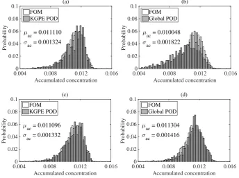
In order to assess the generalization accuracy more fully, we considered a UQ problem for the accumulated contaminant concentrationu¯(x;ξξξ) :=RT₀ u(x, t;ξξξ)dtat the locationxc= (0.5,0.5)T, by consideringξξξto be a random vector distributed according to p(ξξξ) =N(µµµ, σ2I), whereµµµ=

(0.5,0.5)T andσ2= 0.1. The distribution ofu¯(xc;ξξξ)was estimated using Monte Carlo sampling with NM samplesξξξi (this notation is to avoid confusion with the design points) drawn from

p(ξξξ). We setq= 6,n= 80,NM= 3000, and approximatedu¯(xc;ξξξ)with a trapezoidal rule. Fig.6 compares the histograms obtained from kGPE-POD, the global basis method and the FOM, using

m= 10 snapshots. The FOM took55.18h to complete and yielded µac= 0.011087 and σac=

0.001218, obtained from µac= (1/NM)PNi=1Mu¯(x;ξξξ i

) and σac2 = (NM −1)−1PNi=1M(¯u(x;ξξξ i

)−

µac)2. Forr= 10, kGPE-POD exhibited reasonable accuracy with regards toµac(within 0.2 %)

andσac(within 8.7 %), while the global basis method was inaccurate (50 % error inσac). For

m= 10,r= 50, both methods were accurate, with kGPE-POD still providing better estimates of

µacandσac. Form= 100, the results are shown in Fig.7. kGPE-POD was again more accurate for

r= 10, while forr= 30, the two methods exhibited a similar level accuracy.

(b) Burgers equation

We consider a 1-D Burgers equation, with inputsξξξto be defined later:

∂tu+

1 2∂x(u

2

)− 1

Re∂xxu=g(x), x∈ D:= (0,1)

u(0, t) =u(1, t) = 0, u(x,0) =u0(x) := sin(kπx)e−(c1x+c2)

(13)

12

rspa.ro

y

alsocietypub

lishing.org

Proc

R

Soc

A

0000000

..

[image:13.595.129.464.93.545.2]

..

Figure 4.(a) The FOM and (b) the kGPE-POD prediction of the concentration field (mol m−3) for the contaminant

transport model at ξξξ= (0.7382,0.4179)T and t= 0.02s (r≈0.0021). (c) The FOM and (d) the kGPE-POD

predictions atξξξ= (0.7539,0.7461)T_and_t_{= 0}_.₂_s_(r_≈₀_.₀₁₂₇_{). In all cases}_n_{= 80}_,_m_{= 10}_and_q_{= 6}_{. (e) Absolute}

pointwise error for the caseξξξ= (0.7382,0.4179)Tand (f) absolute pointwise error forξξξ= (0.7539,0.7461)T.

whereu(x, t;ξξξ)is the flow velocity,c1, c2∈R,k∈N,Reis the Reynold’s number andg(x)is a source term. We seek a weak solutionu(x, t;ξξξ)∈ V:=H₀1(D)satisfying:

(∂tu, v) +1

2(∂x(u

2

), v) + 1

Rea(u, v) = (g, v) ∀v∈ V (4.5)

wherea(ϕ1, ϕ2) := (ϕ01, ϕ02),ϕ1, ϕ2∈ V, defines a bilinear functional, in which a prime denotes

an ordinary derivative w.r.t. x. The interval D= [0,1] is partitioned intoN+ 1 equally sized subintervals [xi, xi+1], where xi= (i−1)/(N+ 1),i= 1, . . . , d=N+ 2. A standard piecewise

linear basis{ψi(x)}di=1defines the approximating spaceV h

(14)

13

rspa.ro

y

alsocietypub

lishing.org

Proc

R

Soc

A

0000000

..

[image:14.595.127.473.111.250.2]

..

Figure 5.A close-up of (a) the kGPE-POD prediction and (b) the test corresponding to Figs. 4(a) and (b).

Accumulated concentration 0.0040 0.008 0.012 0.016 0.02

0.04 0.06 0.08

0.1 (a)

Probability

FOM KGPE POD

µ

ac = 0.011110

σ

ac = 0.001324

Accumulated concentration 0.0040 0.008 0.012 0.016 0.02

0.04 0.06 0.08

0.1 (b)

Probability

FOM Global POD

µ

ac = 0.010048

σ

ac = 0.001822

Accumulated concentration

0.0040 0.008 0.012 0.016

0.02 0.04 0.06 0.08

0.1 (c)

Probability

FOM KGPE POD

µ

ac = 0.011096

σ

ac = 0.001332

0.0040 0.008 0.012 0.016

0.02 0.04 0.06 0.08

0.1 (d)

Probability

FOM Global POD

µ

ac = 0.011304

σ

ac = 0.001416

Figure 6.Estimated distribution ofu¯(xc;ξξξ)fromNM= 3000MC samples usingn= 80andm= 10: (a) kGPE-POD

withr= 10; (b) global basis withr= 10; (c) kGPE-POD withr= 50; (d) global basis withr= 50.

The FE approximation u(x, t;ξξξ)≈uh(x, t;ξξξ) =Pd_j=1uj(t;ξξξ)ψj(x) leads to the weak formulation: findu=uh(x, t;ξξξ)∈ Vhsuch that (4.5) holds∀v=vh(x)∈ Vh. We also make use of

thegroup (product) approximation[40]:u(x, t;ξξξ)2≈Pd_j=1uj(t;ξξξ)2ψj(x)∈ Vh. Settingu=uhand

vh=ψjin (4.5) we obtain the semi-discrete problem:

d X

i=1

˙

ui(t;ξξξ)(ψi, ψj) +

1 2

d X

i=1

ui(t;ξξξ)2(ψi0, ψj) +

1

Re d X

i=1

ui(t;ξξξ)(ψi0, ψj0) = (g, ψj) (4.6)

together with Pdi=1ui(0;ξξξ)(ψi, ψj) = (u0, ψj), ∀j= 1, . . . , d. Defining the solution vector

u(t;ξξξ) = (u1(t;ξξξ), . . . , ud(t;ξξξ))T, Eq. (4.6) and the initial condition lead to: Mu˙(t;ξξξ) +b(u(t;ξξξ)) + 1

[image:14.595.121.466.288.545.2]

(15)

14

rspa.ro

y

alsocietypub

lishing.org

Proc

R

Soc

A

0000000

..

0.0040 0.008 0.012 0.016

0.02 0.04 0.06 0.08

0.1 (a)

Probability

FOM KGPE POD

µ

ac = 0.010977 σ

ac = 0.001424

0.0040 0.008 0.012 0.016

0.02 0.04 0.06 0.08

0.1 (b)

Probability

FOM Global POD

µ

ac = 0.009970

σ

ac = 0.001668

0.0040 0.008 0.012 0.016

0.02 0.04 0.06 0.08

0.1 (c)

Probability

FOM KGPE POD

µ

ac = 0.011025 σ

ac = 0.001379

0.0040 0.008 0.012 0.016

0.02 0.04 0.06 0.08

0.1 (d)

Probability

FOM Global POD

µ

ac = 0.010938

σ

[image:15.595.122.466.115.377.2]

ac = 0.001322

Figure 7.Estimated distribution ofu¯(xc;ξξξ)fromNM= 3000MC samples withn= 80andm= 100: (a) kGPE-POD

withr= 10; (b) global basis withr= 10; (c) kGPE-POD withr= 30; (d) global basis withr= 30.

where the(i, j)-th elements of the mass and stiffness matricesMandSare given by ψi, ψjand ψ0_i, ψ0_j

, respectively, and thej-th components ofu0andgare(u0, ψj)and(g, ψj), respectively, The nonlinear vector functionb(u(t;ξξξ))arises from the second term in (4.6). We used a Runge-Kutta method with a variable time step to solve the semi-discrete problems in this example.

The coefficients ui,j(ξξξ), j= 1, . . . , d, of the snapshots ui(ξξξ) =u(ti;ξξξ), i= 1, . . . , m, for an arbitrary value of ξξξ are the nodal coefficients in the FEM solution, and thus correspond to

functionsui(x, ξξξ) :=Pdj=1ui,j(ξξξ)ψj(x)∈ Vh. For the definition of the POD basis we chose the

L2(D)norm for optimality; that is,H=L2(D)as defined in Appendix A. A FE approximation

of the POD basis functions {v_jh(x;ξξξ)}d_j=1 is given by vh_j(x;ξξξ) =Pd_i=1vj,i(ξξξ)ψi(x)∈ Vh, j=

1, . . . , d, in which the nodal coefficient vj,i(ξξξ) is thei-th component of the POD basis vector

vj(ξξξ), given by vj(ξξξ) =M−1/2vj(ξξξ), where vj(ξξξ) is an eigenvector of M1/2C(ξξξ)M1/2. Note that L2(D)orthogonality of the basis{vhj(x;ξξξ)}dj=1is equivalent to orthogonality of thevj(ξξξ) w.r.t. hvj(ξξξ),vi(ξξξ)iM:=vj(ξξξ)TMvi(ξξξ). The solution vector is then expanded as in Eq. (2.3):

u(t;ξξξ)≈u(t;ξξξ) =Pr_j=1aj(t;ξξξ)vj(ξξξ) =Vr(ξξξ)a(t;ξξξ), leading to the reduced order model:

˙

a(t;ξξξ) +Vr(ξξξ)Tb(Vr(ξξξ)a(t;ξξξ)) + 1

ReVr(ξξξ) T

SVr(ξξξ)a(t;ξξξ) =Vr(ξξξ)Tg

a(0;ξξξ) =a0(ξξξ) :=Vr(ξξξ)Tu0

(4.8)

Another choice for optimality is H=H10(D) with a(·,·) as the inner product and associated semi-norm|ϕ|1=a(ϕ, ϕ)1/2. The POD eigenvalue problemRT₀ a(u, v)udt=λv(see Appendix A)

leads to the eigenvalue problemC(ξξξ)TSvj(ξξξ) =λvj(ξξξ). The POD basis vectors are then given by

(16)

15

rspa.ro

y

alsocietypub

lishing.org

Proc

R

Soc

A

0000000

..

w.r.t.h·,·iS. In the present example this approach gave almost identical results.

Case 1. In the first example we set g(x)≡0 and k= 1. The inputs were defined as ξξξ= (c1, c2, Re)T∈ X= [2,5]×[0.1,1]×[10,1000]. A total of500inputsξξξj∈ X were selected using

a Sobol sequence and numerical experiments were performed by solving the FOM model (4.7) withd= 64nodes, for eachj= 1, . . . ,500, to obtain the solution vectorsu(ti;ξξξj)and nonlinearity

b(u(ti;ξξξj))at times,ti= 0.25i,i= 1, . . . ,40(m= 40). This yielded the data points (vectorized snapshots) y_j=ηηη(ξξξj) and yfj=ηηη

f

(ξξξj), j= 1, . . . ,500, according to Eq. (3.3). Of the 500 data

points,nt= 300were reserved for testing, and training points were selected from the remaining 200 points. The details of kPCA and GP emulation were as described in the previous example.

Analysis of the normalized errorsfor thenttest cases withn= 160training points showed convergence after q= 8 dimensions. Isomap gave similar results while Diffusion maps was

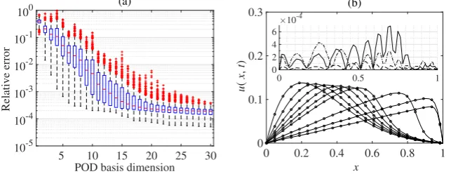
inferior. We used q= 9 (kPCA) in the results presented below. Fig.8(a) shows the results of

5 10 15 20 25 30

10-4 10-3 10-2 10-1 100

Relative error

(a)

x

0 0.2 0.4 0.6 0.8 1

u

(

x

,

t

)

0 0.1 0.2

0.3 (b)

0 0.5 1

×10-4

0 2 4 6

Figure 8.(a) Tukey box plots ofrwith increasingrusing kGPE-POD-DEIM for Burgers model case 1 (n= 180,nt=

300andm= 15). (b) Velocity profiles att= 0,0.5,1,1.5,2,2.5,5,7.5,10s simulated with the FOM (filled circles,

every third node) and kGPE-POD-DEIM (solid lines) for a case withr≈0.041atr= 10. The inset in Figure (b) shows

the absolute pointwise error att= 2.5s (dashed),5s (solid) and10s (dashed dotted).

5 10 15 20 25 30

10-3 10-2 10-1 100

Relative error

(a)

5 10 15 20 25 30

10-3 10-2 10-1 100

Relative error

[image:16.595.130.452.312.436.2]

(b)

Figure 9.Tukey box plots ofr with increasingrfor Burgers model case 1 (nt= 300,m= 40andn= 180): (a)

kGPE-POD; (b) a global basis.

kGPE-POD-DEIM for an increasing r (with s=r). The relative errors converge after r= 30,

[image:16.595.134.451.540.667.2]

(17)

16

rspa.ro

y

alsocietypub

lishing.org

Proc

R

Soc

A

0000000

..

0,0.5,1,1.5,2,2.5,5,7.5,10s from kGPE-POD-DEIM and the FOM for a point (r≈0.041) above

the upper whisker atr= 10in Fig.8(a). The two sets of profiles are very close. The inset in Figure

(b) shows the absolute pointwise error att= 2.5,5and10s. Inspection of the full set of profiles showed that the error grew with time until the front developed, after which the error decayed. The

highest absolute error was around8.62×10−4atx= 0.703,t= 5.65s, for whichu(x, t)≈0.103m s−1. Thus, the maximum error was around 0.84 %.

10 20 30 40 50 60

DEIM basis dimension 10-4

10-3 10-2 10-1 100 101

Relative error

(a)

10 20 30 40 50 60

DEIM basis dimension 10-4

10-3 10-2 10-1 100 101

Relative error

[image:17.595.132.449.202.331.2]

(b)

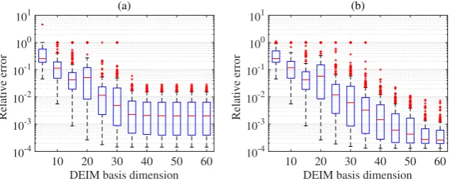
Figure 10.Tukey box plots ofrwith increasingsfor Burgers model case 2 (nt= 300,n= 180andm= 200) using

kGPE-POD-DEIM with: (a)r= 30; and (b)r= 50.

With no approximation of the nonlinearity, a comparison between kGPE-POD and the global basis method exhibited trends similar to those seen in the previous example. Form <30andn≤

200, kGPE-POD required fewer POD vectors to achieve a given level of accuracy; the lower bound

forratr= 10was one order of magnitude smaller for kGPE-POD. Both methods improved with

increasingm, with the global basis method showing a greater improvement, especially in the lower bound forr. Form= 30andn= 180 the results are illustrated in Fig.9, which shows

that aroundr= 28both methods exhibit similar levels of accuracy in terms of the maximum,

minimum and medianr.

Case 2.In a second case we setg(x) = 0.02ex,k= 3andc2= 0.2, with inputsξξξ= (c1, Re)T∈ X=

[2,5]×[10,1000]. As before we selected 500 inputs using a Sobol sequence and ran the FOM to

generate data points, withnt= 300reserved for testing. In this case we used= 128nodes and after inspection of the normalized errorswe setq= 9. In contrast to the previous case, a largem

(m >120) was required for accurate results.

Fig.10shows the trends in the kGPE-POD-DEIM relative errorron thent= 300test points

with increasingsfor two values ofr, usingn= 180andm= 200. For a fixedr, the errors decrease with an increasings. For a fixeds, the errors were seen to decrease as rwas increased up to

a certain value. For higher values of r the solutions became less stable, with a corresponding increase in the error. This was more pronounced for small values ofs. The optimal distribution of

errors (in terms of the median, quartiles and extrema) was achieved for values ofsbetween 5 and 10 higher than the value ofr. Similar results for Burgers equation can be found in, e.g., [45,46].

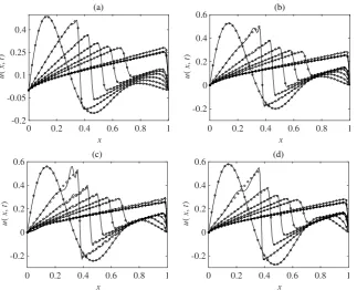
Forr= 30ands= 40, Figs.11(a) and (b) compare the FOM and kGPE-POD-DEIM profiles at t= 0,0.5,1,1.5,2,2.5,5,7.5,10 s. The first of these corresponds to a point near the median

of the relevant box plot in Fig.10(a), while the second corresponds to a point near the upper whisker. Fig.11(c) shows the point with the highest error using the same values ofrands. In this

(18)

17

rspa.ro

y

alsocietypub

lishing.org

Proc

R

Soc

A

0000000

..

0 0.2 0.4 0.6 0.8 1 x

-0.2 -0.05 0.1 0.25 0.4

u

(

x

,

t

)

(a)

0 0.2 0.4 0.6 0.8 1

x

-0.2 0 0.2 0.4 0.6

u

(

x

,

t

)

(b)

0 0.2 0.4 0.6 0.8 1

x -0.2

0 0.2 0.4 0.6

u

(

x

,

t

)

(c)

0 0.2 0.4 0.6 0.8 1

x

-0.2 0 0.2 0.4 0.6

u

(

x

,

t

)

[image:18.595.131.455.101.363.2]

(d)

Figure 11.Velocity profiles predicted by the FOM (filled circles, every third node) and kGPE-POD-DEIM (solid lines) at

t= 0,0.5,1,1.5,2,2.5,5,7.5,10s for Burgers model case 2. (a) A point near the median (r≈0.0022) atr= 30,

s= 40in Figure10(a); (b) a point near the upper whisker (r≈0.0154) atr= 30,s= 40; (c) point with the highest

error (r≈0.0282) atr= 30,s= 40; (d) point with the highest error (r≈0.0072) atr= 50,s= 55in Figure10(b).

case with the highest error is shown in Fig.11(d). In Fig.11(d) we see that the solutions at early

times are more stable. The observed instability is a common feature of POD models [27,41,42].

Stabilization schemes, e.g., alternative inner products, post-processing steps and modification of the underlying model [41,43,44] can be incorporated within the framework we have developed

in order to eliminate or minimize such problems.

5. Conclusions

In this paper we introduced a new POD-ROM method for dynamic, parameter-dependent linear

and nonlinear PDEs. The method uses a Bayesian nonlinear regression to infer the basis for new parameter values and is thus potentially applicable to a broader window of parameter space than

existing methods. Compared to a global POD method, our method requires extra computational effort on each run to diagonalize the snapshot matrix. The actual influence of this is small (as the

UQ in the first example demonstrates) since most of the computational time is spent on solving the ROM. In the examples considered (and others not presented) the global basis method requires

a high value ofrto reach the same level of performance (in terms of the minimum and maximum relative errors) as our method, particularly for low values ofm. At these high values ofr, much

of the benefits of the global basis method as a surrogate model would be eliminated.

Since the method introduced here is a general framework, a number of modifications

(19)

18

rspa.ro

y

alsocietypub

lishing.org

Proc

R

Soc

A

0000000

..

incorporating stabilization schemes, according to different types of problems. The manifold-learning based GP emulator could be treated as a general data-driven technique to interpolate

properties other than the snapshots, as has been accomplished with the method of Amsallem and Farhat [14]. For instance, we could employ it to directly learn the POD basisVr(ξξξ)in Eq. (2.3) or the system matrixAr(ξξξ)in Eq. (2.4), both of which would further reduce the computational time.

Data accessibility.This work does not have any experimental data.

Authors’ contributions. The idea was conceived by AAS, who coordinated the study. The implementation and coding was carried out primarily by WWX and VT. The manuscript was written by AAS. All authors gave final approval for publication.

Competing interests.We have no competing interests. Acknowledgements.We have no acknowledgements to make.

Funding statement. WWX received funding from the Chinese Scholarship Council. AAS received funding from the Engineering and Physical Sciences Research Council, UK (grant Nos. EP/L027682/1, EP/P012620/1 and EP/L018330/1).

Appendix A: Variants of POD

We regardu(x, t;ξξξ)as a realization of a zero-mean random field indexed by(x, t)[2,3,29], with an underlying probability space(Ω,A,P), whereΩ is the sample space,Ais the event space

and Pis a probability measure. It is assumed that u(x, t;ξξξ) is continuous in quadratic mean (q.m.) w.r.t.x(assumption (i)) and stationary w.r.t.t(assumption (ii)). The spatial autocovariance function then takes the form E

u(x, t;ξξξ)u(x0, t;ξξξ)

=C(x,x0;ξξξ), x,x0∈ D. For a fixed t∈[0, T], u(x, t;ξξξ)defines aone-parameterrandom field indexed byx∈ D[29]. Sample paths (fixedω∈Ω) are deterministic functionsu(·, t;ξξξ) :D →R. By assumption (i),u(·, t;ξξξ)∈L2(D)for eacht∈[0, T]

so that u(x, t;ξξξ)∈L2(0, T;L2(D)). KL theory [31] for a fixedtshows thatu(x, t;ξξξ)is the q.m. limit of the sequence of partial sumsSM=PMi=1ai(t;ξξξ)vi(x;ξξξ), with randomness entering only throught. Thevi(x;ξξξ)form anL2(D)orthonormal basis and are given by the eigenfunctions of an operatorC:

Cvi(x;ξξξ) := Z

D

C(x,x0;ξξξ)vi(x0;ξξξ)dx0=λ0ivi(x;ξξξ) i∈N (A1) with corresponding real, positive eigenvalues λ0i(ξξξ)> λi+10 (ξξξ) ∀i∈N. The coefficients satisfy E[ai(t;ξξξ)] = 0 andE[ai(t;ξξξ)aj(t;ξξξ)] =λi0(ξξξ)δij and sincet is arbitrary, they can be interpreted

as uncorrelated random processes. The expectation operator E[X] =R_ΩX(ω)P(dω), is approximated by a time average (obtained from the snapshots), assuming ergodicity.

The ‘optimality’ of the basis {vi(x;ξξξ)}i∈N can be interpreted in two equivalent ways. For

an arbitrary orthonormal basis{ϕi}∞i=1ofL2(D), Pr

i=1E[(u, vi)2] =Pri=1λ

0

i> Pr

i=1E[(u, ϕi)2], ∀r∈N, i.e., a generalized ‘variance’ maximization. Equivalently we minimize the ‘error’E[||u− Pr

i=1aiϕi||2] =||u−Pri=1aiϕi||2L2_(0,T;L2₍_D₎₎ over orthonormal bases {ϕi}∞i=1. These results carry over to the finite-dimensional setting described below, in which case orthonormality is defined w.r.t. an inner product inRd. More generally, we seekmin{ϕi}||u−

Pr

i=1aiϕi||2L2_(0,T;_H₎ for any separable Hilbert spaceH. In this case the POD basis is defined by theH-orthonormal eigenfunctionsv(x)∈ Hof the operatorRv:=E[u(u, v)H] =

RT

0 u(u, v)Hdt. ForH=L 2

(D),R=

(20)

19

rspa.ro

y

alsocietypub

lishing.org

Proc

R

Soc

A

0000000

..

Defining quadrature points {ti}m_i=1 and (equally spaced) {xi}d_i=1, problem (A1) can be approximated numerically using a midpoint rule:C(ξξξ)vi(ξξξ) =λi(ξξξ)vi(ξξξ)for eigenvectorsvi(ξξξ)∈ Rd and positive (decreasing) eigenvalues λi(ξξξ), i= 1, . . . , d. This is a principal component

analysis (PCA) with spatial variance-covariance matrix C(ξξξ) =U(ξξξ)U(ξξξ)T≈E[u(t;ξξξ)u(t;ξξξ)T], in which U(ξξξ) := [u1(ξξξ). . .um(ξξξ)]. The j-th component vi,j(ξξξ) of vi(ξξξ) can be identified with vi(xj;ξξξ) and the (i, j)-th entry of C(ξξξ) approximates C(xi,xj;ξξξ) as the time average

(1/m)P

ku(xi, tk;ξξξ)u(xj, tk;ξξξ). Other interpolation procedures for (A1) can also be used. For instance, in the FE formulation (section4(b)) we can approximateu(x, t;ξξξ)andvi(x;ξξξ)using a standard piecewise linear basis {ψi(x)}i=1d ⊂L2(D), which leads to C(ξξξ)Mvi(ξξξ) =λi(ξξξ)vi(ξξξ), where M is a mass matrix with entries Mij= (ψi(x), ψj(x)). Defining v(ξξξ) =M1/2v(ξξξ) we obtainM1/2C(ξξξ)M1/2v(ξξξ) =λ(ξξξ)v(ξξξ). The eigenvalues/eigenvectors pairs{(vi(ξξξ), λi(ξξξ))}di=1of M1/2C(ξξξ)M1/2yield the POD basis vectorsvi(ξξξ) =M−1/2vi(ξξξ)in the desired order.

The method of snapshots is used when md. The temporal autocovariance function

K(t, t0;ξξξ) =R_Du(x, t;ξξξ)u(x, t0;ξξξ)dxdefines an operatorKai(t;ξξξ) := RT

0 K(t, t

0_;_ξξξ₎_a

i(t0;ξξξ)dt0. The eigenfunctionsai(t;ξξξ)ofKare equal to the POD coefficients, and the eigenvalues are identical

to those of C. Using E[ai(t;ξξξ)aj(t;ξξξ)] =λ0i(ξξξ)δij, the POD modes are given by vi(x;ξξξ) =

(1/λ0_i(ξξξ))RT₀ u(x, t;ξξξ)ai(t;ξξξ)dt. The discrete form (in space and time) of the eigenvalue problem isU(ξξξ)TU(ξξξ)ai(ξξξ) =λiai(ξξξ), whereK(ξξξ) :=U(ξξξ)TU(ξξξ)is a kernel matrix with entries Kij=

ui(ξξξ)Tuj(ξξξ), i.e., the space-discrete form of K(ti, tj;ξξξ). The eigendecomposition is K(ξξξ) = A(ξξξ)ΛΛΛ(ξξξ)A(ξξξ)T, whereΛΛΛ(ξξξ) =diag(λ1(ξξξ), . . . , λm(ξξξ)) and the columns ofA(ξξξ) are given by

the ai(ξξξ). The j-th component ai,j(ξξξ) of ai(ξξξ) approximates ai(tj;ξξξ) yielding the discrete-time approximation vi(x;ξξξ) = (1/λi(ξξξ))Pmj=1u(x, tj;ξξξ)ai,j(ξξξ), i.e., a linear combination of the snapshots. In the fully-discrete case, using the normalization ai(ξξξ)7→a0i(ξξξ)/

p

λi(ξξξ), we

obtainvi(ξξξ) =U(ξξξ)a0i(ξξξ)/ p

λi(ξξξ). These relationships are also evident from the singular value

decomposition (SVD) ofU(ξξξ), that isU(ξξξ) =A0(ξξξ)ΛΛΛ(ξξξ)1/2V(ξξξ)T, where the columns ofV(ξξξ)are

given by thevi(ξξξ)and the columns ofA0(ξξξ)are given by thea0i(ξξξ). In this context, the columns ofA0(ξξξ)andV(ξξξ), given respectively by the eigenvectors ofK(ξξξ)andC(ξξξ), are referred to as left

and right singular vectors. It is straightforward to show thatvi(ξξξ) =kU(ξξξ)a0i(ξξξ)fork∈R. Thus we recover the earlier relationship by takingk= 1/pλi(ξξξ)to normalize thevi(ξξξ).

Appendix B: Kernel PCA and an inverse mapping

Kernel PCA on the training data. Given training datay_i=ηηη(ξξξi)∈ O, i= 1, . . . , n, kPCA [35] defines a map φφφ:O →F, where F is a feature space. The mapped points are centred by

e φ φ

φ(y_i) =φφφ(y_i)−φφφ, whereφφφ=n−1Pn_j=1φφφ(y_j). The ’tilde’ symbol is used throughout to denote the corresponding quantity centred in feature space. kPCA then applies linear PCA to the sample covariance matrixCF=n−1Pni=1φφφe(y_i)φφeφ(y_i)

T

. The mapφφφ(·)is specified implicitlyviaa kernel

function k(yi,yj) =φφφ(yi) T

φ φ

φ(yj), e.g., the Gaussian kernel k(yi,yj) = exp (−||yi−yj|| 2

/s2),

where sis a scale factor. Defining a kernel matrix K= [Kij=k(yi,yj)] n

i,j=1, a centred kernel matrix is given byKe=HKH, whereH=I−n−111T and1=n−1(1, . . . ,1)T∈Rn.

We assume that dimF> n without loss of generality. The orthonormal eigenvectors w

of CF are linear combinations of φφeφ(y_i) and the eigenvalue problem for C_F is equivalent to the eigenvalue problem for n−1Ke [35], which possesses orthonormal eigenvectors αααi=