Kinematic calibration of a 3 DOF spindle head using a double ball bar

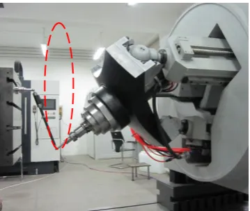
warwick.ac.uk/lib-publications

Original citation:

Tian, Wenjie, Yin, Fuwen, Liu, Haitao, Li, Jinhe, Li, Qing, Huang , Tian and Chetwynd, D. G..

(2016) Kinematic calibration of a 3-DOF spindle head using a double ball bar. Mechanism and

Machine Theory, 102 . pp. 167-178.

Permanent WRAP URL:

http://wrap.warwick.ac.uk/82166

Copyright and reuse:

The Warwick Research Archive Portal (WRAP) makes this work by researchers of the

University of Warwick available open access under the following conditions. Copyright ©

and all moral rights to the version of the paper presented here belong to the individual

author(s) and/or other copyright owners. To the extent reasonable and practicable the

material made available in WRAP has been checked for eligibility before being made

available.

Copies of full items can be used for personal research or study, educational, or not-for-profit

purposes without prior permission or charge. Provided that the authors, title and full

bibliographic details are credited, a hyperlink and/or URL is given for the original metadata

page and the content is not changed in any way.

Publisher’s statement:

© 2016, Elsevier. Licensed under the Creative Commons

Attribution-NonCommercial-NoDerivatives 4.0 International

http://creativecommons.org/licenses/by-nc-nd/4.0/

A note on versions:

The version presented here may differ from the published version or, version of record, if

you wish to cite this item you are advised to consult the publisher’s version. Please see the

‘permanent WRAP URL’ above for details on accessing the published version and note that

access may require a subscription.

Kinematic Calibration of a 3-DOF Spindle Head using a Double Ball Bar

Wenjie Tiana,b_{, Fuwen Yin}b_{, Haitao Liu}b,_{*, Jinhe Li}b_{, Qing Li}b_{, Tian Huang}b,c_{, Derek G. Chetwynd}c a_{School of Marine Science and Technology, Tianjin University, Tianjin 300072, China}

b_{Key Laboratory of Mechanism Theory and Equipment Design of The State Ministry of Education, Tianjin University, Tianjin}

300072, China

c_{School of Engineering, The University of Warwick, Coventry CV4 7AL, UK}

Abstract:

This paper presents a simple and effective approach for kinematic calibration of a 3-DOF spindle head developed for high-speed machining. This approach is implemented in three steps, (i) error modelling that allows the geometric errors affecting the compensatable and uncompensatable pose accuracy to be classified; (ii) identification of the geometric errors using a set of distance measurements acquired by a double ball bar (DBB) with a single installation; (iii) design of a linearized error compensator for real-time error implementation. Experimental results on a prototype machine show that the compensatable pose accuracy can significantly be improved by the proposed approach.

Keywords: Error modelling, Kinematic Calibration, Parallel mechanism

1. Introduction

Machining large structural components with high metal removal rates is a challenging issue in the aircraft industry [1]. Conventionally, it requires a huge gantry 5-axis machine tool, weighing many tons and having a large footprint. A promising alternative is to use one or more machining stations moving along a long reference track that forms the base of a manufacturing system, where each station is a parallel kinematic machine (PKM) configured as a multiple-axis spindle head. This has been demonstrated by the very successful application of the Sprint Z3 head [2]. Motivated by this idea, a new spindle head, named the A3 head, has been designed and developed [3,4] (see Fig.1); its topological structure is a 3-RPS parallel mechanism having movement capabilities of one translation and two rotations (1T2R).

Geometric accuracy is one of the important performance specifications of the PKM based spindle heads as the high rigidity and high accuracy are the essential requirements [5]. It is well recognized that, provided that the manufacturing and assembly processes ensure sufficiently repeatability, a practical and economical way for enhancing pose accuracy is the kinematic calibration by software [5-7], a process by which the actual kinematic parameters can be estimated so as to modify the inverse kinematic model residing in the CNC controller. The critical step in such a calibration is to effectively and accurately estimate the measurement residuals, i.e., the discrepancies between the measured and the computed poses of the cutting tool.

In comparison with self or autonomous calibration in the joint space that minimizes the discrepancies between the measured and computed values of the active, passive and/or redundant sensors in the joint space, external calibration in the task space has been intensively investigated in the past decades. The approaches can be basically classified into two categories, i.e., the coordinate-based approach and the distance-based approach, heavily dependent upon the type of acquirable data. The coordinate-based approach deals with the identification problem by minimizing the discrepancies between the measured and computed values of the full/partial position and orientation of the end-effector directly, or the absolute coordinates of three or more reference points fixed on the end-effector. For example, Masory [8] and Zhuang [9] used a theodolite to measure the positions of three points on the platform of a Stewart platform and extracted the position and orientation information from these coordinate measurements. Vischer [10] measured the position errors of a Delta robot by attaching the end-effector to the probe of a 3D coordinate measuring machine, and the orientation errors by using three perpendicularly placed linear digital probes. Fan [11] investigated the calibration of a 3-RPS parallel mechanism by measuring the orientation errors using an inclinometer and the positioning errors of a reference point using an X-Y table. Huang [12,13] studied the same problem by measuring the orientation errors of the end-effector using a specially designed fixed angle gauge and the positioning errors of a reference point using three perpendicularly placed dial indicators. The distance-based approach deals with the identification problem by minimizing the discrepancies between the measured and computed values of a set of distances between two or more points. This approach is more cost-effective than the coordinate based approach because it directly uses a contact 1-dimemsional measurement system such as a linear variable differential transducer or a DBB. Then, the partial pose information can be recorded when the end-effector moves along several prescribed paths within the workspace. The distance measurements can also be extracted indirectly from the absolute coordinates of one or more reference points on the end-effector at different configurations. For example, Ota [14] investigated the calibration problem of a 6-DOF parallel kinematic machine (PKM) known as HexaM using the data acquired by a DBB. Yukio [15] proposed an effective approach that employed a lower band FFT filter to improve the signal/noise ratio of circular measurements acquired by a DBB. Patel [16] presented a new calibration method that uses extra "legs", e.g., a simple length measuring device or a string potentiometer, to identify the kinematic parameters of a hexapod-type PKM. Nubiola

[17,18] proposed a novel measurement system comprising a single DBB and two custom-made fixtures. One fixture is attached to the base and the other to the end-effector, and each having three magnetic cups. It is possible to use the DBB to measure six distances between the magnetic cups on the tool fixture and the magnetic cups on the base fixture, and thus calculate the pose with high accuracy. However, the process of the measurements is manual and labor intensive, and only suitable for small industrial robots, particularly if a relatively small workspace is of interest. Many other researches also have been carried out using distance-based approach [19-22]. Compared with the coordinate-based approach, the advantages of the distance-based approach are that the obtained data is independent on the selection of reference frame and it is unnecessary to identify the errors describing the rigid body motion of robot frame relative to the world frame because robot localization can be carried out afterwards according to the environmental context.

Driven by the practical need to ensure machining accuracy, this paper presents a distance-based approach for kinematic calibration of the A3 head. It concentrates upon three key issues: 1) formulation of an error model that is able to distinguish the geometric errors affecting the compensatable pose accuracy from those affecting the uncompensatable pose accuracy; 2) identification of a full set of errors using distance measurements acquired by a DBB; and 3) development of a linear error compensator for real-time implementation. Experiments carried out on a prototype machine verify the effectiveness of this approach.

2. Error Modelling

2.1. Inverse displacement analysis

Fig.1 shows the 3D model of the A3 head, which consists of a moving platform, a base, and three identical RPS limbs. Here, R, P and S represent revolute, actuated prismatic and spherical joints, respectively. Driven by three independent servomotor lead-screw assemblies, the platform achieves three degrees of freedom: one translation along the z axis and two rotations about the x and y axes. A spindle can be mounted on the platform to implement high-speed milling. For more information about mechanical design of the A3 head, please refer to [4].

Fig.1. 3D model of the A3 head.

Fig.2. Schematic diagram of the A3 head.

Fig.2 shows the schematic diagram of the A3 head. In order to implement geometric error modelling, attach the reference frame Bxyzto the base with Bat the centre of the equilateral triangleB B B_{1 2 3}, its z axis perpendicular to

1 2 3

B B B

 , and its x axis parallel toB B_{2 3} . Then, place a body fixed frameB_ix y z_{i i i}on the ith (i1, 2,3) limb with the

i

 A

1

A

2

A

3

A

B

1

B

2

B

3

B

x y

z

u v

w a

1 a

p

r

b

1

b

1

x

1

z

1 2,1

q s

1

y

P c

1,1

s

i



Servomotor

Limb body

Closed frame

Ball screw

Revolute joint Block unit Spindle Platform Spherical

joint

Base Guideway

z y

i

x andz_iaxes coincident with the nominal axes of the revolute and prismatic joints, and BB_i xi. The body-fixed

frame A uvw is attached to the platform using rules similar to those for Bxyz.

In Bxyz, the nominal position vector r_p



x y z



Tof the pointPrepresenting the cutting tool point (TCP) can be expressed as

2,

p

 

i

q

i i



i

r

b

s

a

,a_i Ra_0i,i1, 2,3 (1)





cos cos sin cos sin cos sin sin cos cos sin sin sin cos cos cos sin sin sin cos cos cos cos sin

sin sin sin cos cos

           

           

    

  

 

 

_     _

 

 

R u v w

where a_0i



acos_i asin_i c



Tis the nominal position vector pointing from P toA_ievaluated in A uvw ,





T

cos sin 0

i b i i

b is the nominal position vector pointing from BtoB_ievaluated in Bxyz, with aAAi,

i

bBB ,cAP and _i 2π(i1) / 3 π/2 ;q_iand

s

_2,iare the nominal limb length and unit vector pointing from B_ito

i

A ;Ris the orientation matrix of A uvw with respect to Bxyzwith  , andbeing the Euler angles of precession, nutation and body rotation, respectively. Taking ,



and zas three generalized coordinates, the other three dependent coordinates (also referred to as the parasitic motions) can be obtained by solving the constraint equations



ra_i



Ts_1,i 0(i1, 2,3) imposed by the revolute joints



1 cos



sin 2 sin sin 2

a

x 





c





,



1 cos



cos 2 cos sin 2

a

y 





c





,   (2)

wheres_1,i  



sin_i cos_i 0



Tdenotes the unit vector of the x_iaxis. Therefore, two independent motions along the

xandyaxes should be added to compensate the parasitic motions, which in conjunction with the A3 head forms a 5-axis machine tool.

Given three independent motions  ,  and z, R and r_p can be determined using Eqs.(1) and (2). Then, by Eq.(1), the inverse position problem can be solved as

i p i

q  r  b a_i , 2,

p i

i

i

q

  r b ai

s , i1, 2,3 (3)

2.2. Formulation of a linearized error model

We here draw on screw theory to develop a linearized error model that can readily be employed for the geometric error identification and pose error compensation. Taking small perturbations on both sides of Eq.(1) leads to





2, 2, 1, 2, 1, 2, 0

p i qi i iqi i i i iqi i i i i

    r b s   s s s   s s     α a R a , i1, 2,3 (4)

where  r_p



x y z



Tand  α



_x _y _z



Tdenote the positioning error vector of P, the TCP, and the angular error vector of the platform;b_i and a_0idenote the position error vector ofB_ievaluated in Bxyzand the position error vector of A_ievaluated in A uvw ; q_iand

s

1,i are the length error and the nominal unit vector of the

i

x axis of limb i; and _iand_iare the angular errors of limb i about the x_iand they_iaxes, respectively. Taking dot products on both sides of Eq.(4) with each of

s

2,iand

s

1,ithen leads to















 





T

T T

2, 2, 2, 0

T

T T

1, 1, 1, 0

i p i i i i i i

i p i i i i i i i

q

q d d 

         

         

s r a s α s b R a

s r a s α s b R a

, i1, 2,3 (5)

wheredis the nominal distance betweenA A A_{1 2 3}andB B B_{1 2 3}at the initial (home) configuration. Writing it in this form, all the geometric errors to be identified become dimensionally homogeneous. Rewriting Eq.(5) in matrix form now provides the geometric error model of the A3 head with respect to Bxyz.

p

p p      _    r x α , T  

A W B, W



W_a W_c



2,1 2,2 2,3

1 2,1 2 2,2 3 2,3

a

 

  _{  } 

 

 

s s s

W

a s a s a s ,

1,1 1,2 1,3

1 1,1 2 1,2 3 1,3

c

 

  _{  } 

 

 

s s s

W

a s a s a s





T T

3 2, 2,

T T

1, 1,

diag diag

diag diag diag

i i

i i q di

 _ _  _ _ 

 



 _ _  _ _ 

 

E s s R

B

s s R

0 0 0 d     _             q b p a β , 1 2 3 q q q        _{ } _    q , 1 2 3        _{ } _    b b b b , 01 0 02 03        _{ } _    a a a a , 1 2 3           _{ } _    β

whereE₃is an identity matrix of order 3. It can be seen that p contains 24 independent geometric errors, including the home errors (the encoder offsets) of the limbs, the position errors of the base and the platforms, and the orientation errors of the prismatic and revolute joint axes.

3.Error Identification using a DBB

The geometric error model developed in Section 2.2, is now used to build a method for error identification using a double ball bar (DBB). To do this, Eq.(6) is partitioned into the form

p r

  

r

A p

,  α A_p (7)

As shown in Fig.3, the DBB connects the spindle and the work table with two precision chrome steel balls and two magnetic tri-hedral cups, which can usually provide a very high accuracy of 0.1 μm. One end of the DBB is attached to the spindle (P) using a magnetic cup while the other end is mounted on the work table (S). The machine is programmed to moving along circular paths, and the radial errors between the actual travel path of the tool and its nominal path are measured and recorded by the DBB.

Fig.3. Pose error measurement of the A3 head using a DBB.

Let r_s be the nominal position vector of the centreSof the stationary magnetic cup, and

r

p j k, , be the nominal

position vector of the centre P of the movable magnetic cup at thekthconfiguration in thejthcircle. Thus, the loop closure equation gives

, , ,

ˆ

_{j k p j k s}

l

n



r



r

, j1, 2, ,m, k1, 2, , n (8)

whereland

n

ˆ

j k, are the nominal length of the DBB and the nominal unit vector pointing fromStoP.

By considering the geometric errors, the actual positions of point Sand point P are expressed by point Sand point P (see Fig. 4(a)). Let   r_s r_s r_s,



r

p j k, ,



r

p j k



, ,



r

p j k, , , and

l

 

n

ˆ

j k,



r

p j k



, ,



r

s



(where l and

n

ˆ



j k, are the

actual length of the DBB and the unit vector pointing from point S to point P). By making a pure translation of

S P  by vector r_ssuch that point S coincides with point S (see Fig.4(b)) and lettingnˆ_{j k,} nˆ_{j k,} nˆ_{j k,} be the tangential variation of

n

ˆ

j k, and   l l l be the variation of DBB length, then



r

p j k, ,

 

r

sshown in Fig.4(b) can be

expressed as

S A

, , p j k

r

P ,

ˆ_{j k}

ln u v w B x y z s r O X Y Z   z S P

Ball at tool nose Ball on work table

DBB

Spindle





, , ˆ, , ˆ, ˆ , , ˆ , ˆ ,

p j k s l j k lj k j k l j k lj k j k j k

r    r n   n  n   n  n (9)

Fig.4. Geometric errors of DBB system.

Taking dot products on both sides of Eq.(9) withnˆ_{j k,} and noticing thatnˆTj k_, nˆj k_, 0leads to





T

, ˆ , , ,

j k j k p j k s

l

 n r  r (10)

Note that     r_s r_s scan be decomposed into two components: the first term,r_s, is caused by the geometric errors of the mechanism itself; and the second term, s, is induced by the installation error of the stationary cup. Also, by using Eq.(7), r_sand



r

_{p j k, ,} can be expressed as

,

s



r s

 

r

A



p

,



r

p j k, ,



A

r j k, ,



p

(11)

Substituting Eq.(11) into Eq.(10), leads to

, ,

,

1,2,

, ,

1,2,

,

j k j k

l

j

m k

n





h



ρ





(12)

where





T

, ˆ, , , , 3 ,

i k j k r j k r s

  

 

 _   _{    }

  

p

h n A A E ρ

s

The pose error of the cutting tool with respect to the workpiece frame OXYZcan be decomposed into two components: the first component is the pose errors of the cutting tool relative to Bxyz; and the second component is the rigid body misalignments of Bxyzrelative to OXYZ. Then, the geometric errors can be identified by using either of the two following approaches, depending upon different ways of specifyingBxyz.

Approach 1: Let A uvw be parallel to Bxyz at the initial (home) configuration. Then, the rigid body misalignments of Bxyzrelative to OXYZ can be specified by measuring the rotational misalignments of

A uvw relative toOXYZ, and by assigning the translational misalignments of A uvw relative to OXYZto be zero since the home positions along the x and y axes can be set arbitrarily. These considerations result in six constraint equations



r0 3 3



r0

  

 _{ } 

  

p

A h ρ

s

0 0 , 0



0 3 3



0

  

  _{ } 

  

p

α A h ρ

s

0 (13)

Combining Eq.(13) with Eq.(12) leads to6



m n



linear algebraic equations.

 l H ρ (14)

where

P S

, , p j k r

, , p j k

r

B

s r

,

ˆ_{j k} ln

s

r

s r

, , p j k



r ,

ˆ_{j k} l n

P S

, , p j k s

r  r ,

ˆ_{j k}

n ,

ˆ_{j k}

n

,

ˆ_{j k} l n

,

ˆ_{j k} ln

,

ˆ_{j k}

n lnˆ_{j k,}

,

ˆ_{j k} l 

n

(a)

0 1 2 m                  H H H H H

, 0 0

0 r         h H h , ,1 ,2 , j j j j n                h h H h , 6 1 1 2 m    _             _    l l l l 0 , ,1 ,2 , j j j j n l l l    _          _   

l , j1, 2, ,m

According to [23], the necessary conditions for ρ to be identifiable are: (i) the A3 head must experience all controllable DOF, i.e. the translation along the z axis and rotations about the x and y axes, meaning that the distance measurements between S and P must be made along at least two testing circles parallel to thexyplane; (ii) the number of measurements along the two circles must satisfy 6



m n 



dim(ρ). Then, the geometric errors defined in the OXYZcan be estimated by means of linear least square algorithm.

+

 

ρ H l



, _H+ 



_{H H}T



1_HT ₍₁₅₎

Approach 2: It should be pointed out that not all of geometric errors are identifiable using a DBB since the metrology cannot provide the information necessary to describe the rigid-body transformation between the workpiece frame OXYZ and the reference frame Bxyz. Nevertheless, this problem can be solved by presenting the

OXYZ and Bxyz in such a way that: (i) B₁, B₂ and B₃ lie in the xy plane; (ii) the x axis is parallel to

2 3

B B ; (iii) the y axis contains B₁. In this way, the rigid body motions of Bxyzrelative toOXYZ could be eliminated by specifyingBxyzsuch that

1

Δb_x 0,

Δ

b

₂y



Δ

b

₃y



0

, Δb1z Δb2z Δb3z 0 (16)

Note that other choices can also achieve this condition. This treatment allows the number of geometric errors being identified to be reduced from 24 to 18, i.e.



_{T T T}



T

1y 2x 3x 0

b b b d

  p q a β (17)

Consequently, Eq.(15) becomes

+

 

ρ H l



(18)

where 1 2 m              H H H H , ,1 ,2 , j j j j n                h h H h , 1 2 m    _     _{ }      l l l l , ,1 ,2 , j j j j n l l l    _          _   

l , j1, 2, ,m

The geometric errors defined in this specifically definedBxyzcan be estimated if the above mentioned conditions are fulfilled and



m n



dim(ρ)is satisfied. Note that once the pose errors with respect to Bxyz are compensated, the frame A uvw at the initial (home) configuration is parallel to Bxyz. Hence, the rigid body misalignments of

Bxyzrelative to OXYZcan be eliminated or minimized during the assembly process by measuring the angular misalignments of A uvw relative to OXYZ.

4. Pose Error Compensation

In this section we develop a linearized error compensator for the three compensatable pose errors. Here, we choose the translational error along thezaxis, and the precession and nutation angular errors as the compensatable pose errors of the A3 head. This is because the angular error about the spinning axis of the cutting tool does not affect the accuracy in the 5-axis machining, and the translational errors along thexandyaxes can be compensated by the corresponding drives.

It is easy to prove that there is a linear map between the angular errors of the cutting tool evaluated in Bxyz

and those evaluated by the “z-x-z” Euler’s angle conventions,

0 cos sin sin 0 sin cos sin

1 0 cos

  

  



 

 

_  _

 

 

 ,   ε



  



T

where  ,



and denote the angular errors of the precession, nutation and body rotation. Clearly, there are infinite combinations of andthat satisfy_z     when



0, or when  _x 0and



y



0

, where x

and



_yrepresent the orientation angles of the cutting tool about the x and y axes. Therefore, we may set  0when 0



 in order to obtain a unique solution. This requirement can by fulfilled by assigningΔa₀₁x 0. Substituting Eq.(19) into Eq.(5), yields a particular form of Eq.(6) as

p

  

x

A p

(20)

p p



 

  _ 

 

r x

ε ,

T 



A W B, W 



W_a W_c



,   ε



  



T



2,1





2,2





2,3



T T T

1 2,1 2 2,2 3 2,3

a

 

  _{  } 

 

 

s s s

W

a s a s a s







,













1,1 1,2 1,3

T T T

1 1,1 2 1,2 3 1,3

c

 

  _{  } 

 

 

s s s

W

a s a s a s







p



x

has two partitions associated respectively with the compensatable and uncompensatable pose errors of the cutting tool, i.e.

pa p

pc

    _{ }   

x x

x ,





T

pa z  

x     , x_pc  



x y 



T (21)

Then, performing matching elementary row transformations on T

W and partitioning the resultantT gives the form

T

Elementary row operation: a aq ap

cq cp

c

 _   

    

   

T T

T

W T

T T

T (22)

Now, we modify the nominal limb lengthsqbyq_m  q q_msuch that Eq.(21) can be written as

pa a aq ap m

pc c cq cp



 

         

_{ }           

   

x T T T q

B p

x T T T 0 (23)

Hence, an error compensatorq_mcan be designed by forcing the compensatable pose error vector to be zero, namely,

pa





x



0

1

m aq a



q  T T B p (24)

Furthermore, the uncompensatable errors of the A3 head after error compensation can be predicted by



1



pc c cq aq a





x  T T T T B p (25)

5. Experimental Validation

In order to validate the approach proposed in this article, calibration experiments were carried out on a test bed (see Fig.5) which is composed of anA3 head and an X-Y table driven by an IPC+PMAC CNC controller. The orientation movement capability of the A3 head is



 0 40and   0 360and the stroke is s0 200 mm along the z axis. The translational ranges of the X-Y table are X0 800 mmand Y 0 800 mm, respectively. The nominal dimensions of the A3 head are given in Table 1.

Table 1 Dimensional parameters of the A3 head.

a b d c

[image:9.595.175.422.60.231.2]

Fig.5. The test bed of the 5-axis hybrid machine tool.

5.1. Test trajectory planning

To obtain the best signal/noise ratio, it is preferable to place the test configurations as near as possible to the task workspace boundary, because the pose errors are more sensitive to the errors there than when nearer to the centre of workspace [24]. Thus, a DBB with nominal length of 300 mmand measuring accuracy of 0.5 μmwas used so as to measure the distance errors between the TCP and the stationary magnetic cup mounted on the X-Y table when the cutting tool moves along circular paths having large nutation angles.

In order to determine adequate distance measurements for kinematic identification, let m be the number of the selected testing circles, evenly distributed along the stroke range of s0 200 mm.Also, letnbe the number of testing points evenly spaced around each circle. Then, the condition number



of the identification matrix Hwas used as an index to minimize the total number of distance measurements.Fig.6plots



versus m2 ~ 5 _and n12 ~ 20. It shows that



_{varies only slightly with}m, but decreases rapidly up to n15and nearly keeps unchanged when

15

[image:9.595.201.403.456.607.2]

n . So, it is reasonable to choosem2andn15as the minimum set of distance measurements without affecting the identification accuracy, leading to the locations and orientations for the prescribed two testing circles given in Table 2.

Fig.6. Variations of ( H vs) . m and n.

Table 2 The locations and orientations of two testing circles.

z  

Testing circle1 80 mm 28.41°~32.85° 0~360° Testing circle2 200 mm 32.18°~38.34° 0~360°

5.2. Calibration strategy

Considering that the pose errors caused by the home errors,q, are usually much larger than those caused by the other errors, the kinematic calibration was conducted in two steps so as to reduce the cut-off errors arising from the linearization. In the first step known as rough (home) calibration,



x



pagiven in Eq.(23) was assumed to be merely

caused by the home errors (encoder offsets)q. Hence, qwas roughly identified by q H+land



x



pawas

12 14

16 18

20 2

3 4

5 0.5

1 1.5 2

x 104

m n

 4 10



( )

 H interpolation

O Y

Z

X

B y

z

X-Y Table _{3-RPS Mechanism}

Test bed

[image:9.595.162.429.650.686.2]

compensated by assigning qm qin an iterative manner until the estimated q converged to within a specified

threshold. Then, the fine calibration was carried out by taking into account the full set of errors.

5.3. Implementation

[image:10.595.208.388.218.370.2]

Fig.7 shows the machine undertaking distance measurements with the DBB according to the optimized testing circles given in Table 1 and two-step strategy addressed in Section 5.2. Prior to the measurement, the machine was run for an hour to achieve a relatively stable thermal status. The environment temperature fluctuation was controlled within 22.90.6 C during the experiment. In the measurement, the TCP moved with a feed rate of 300 mm/minaround a testing circle and the length error at a testing point on the circle was measured six times, three times clockwise and three times anticlockwise. The mean value was then retained. In practice, the calibration process ran three times for the home errors to converge to q₁ 7.812 mm, q₂ 9.237 mm, q₃ 6.690 mm. This was followed by the full set errors identification using Eq.(18), leading to the results presented in Table 3.

Fig.7. Distance measurements using a DBB.

Table 3 The identified geometric errors.

Errors Limb 1 Limb 2 Limb 3

i

q

 (mm) −1.0104 −1.4540 −0.7043

ix

b

 (mm) --- −0.7453 −0.0949

iy

b

 (mm) −0.8735 --- ---

0ix

a

 (mm) --- 0.0833 0.1023

0iy

a

 (mm) 1.0215 1.0750 0.9646

0iz

a

 (mm) 0.7907 1.5004 −0.4216

i



 (deg) −0.4485 −0.7084 −0.5500

x

s

 (mm) 0.0144

y

s

 (mm) −0.0104

z

s

 (mm) −0.0097

In both the rough and fine calibration, the nominal limb lengths, q, at a given configuration was modified byqm,

determined by Eq.(24). This allows ,



andzto be compensated, and



x

,



y

and





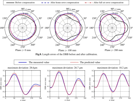
to be estimated at the same time by Eq.(25). Fig.8 shows the length errors measured on the DBB before and after error compensation for three circles located at z0 mm, z100 mm andz200 mm, respectively. The length errors are dramatically reduced after the home calibration, particularly as the z coordinate of the TCP takes large values. However, due to the existence of the uncompensatable pose errors



x

and



y

, the length errors, although further reduced, did not vanish even after



[image:10.595.186.409.417.583.2]

[image:11.595.63.532.60.417.2]

Fig.8. Length errors of the DBB before and after calibration.

Fig.9. Discrepancy between the predicted and measured length errors of the DBB after fine calibration.

5.4. Verification using a laser tracker

As an independent test of the effectiveness of the distance-based calibration, a reference frameOmx y zm m mwas

generated at the home position via curve fitting using the data acquired by a laser tracker at six evenly spaced points on the platform, as shown in Fig.10. The measurement uncertainty and maximum resolution of the laser tracker are 0.005 mm and 0.001 mm, respectively. A body fixed frame Om x y zm  m mwas placed coincident withOmx y zm m mat the

home position. Given  0 ~ 360,



 35 and z100 mm, Fig.11 shows the positioning errors of Omalong the z axis and the orientation errors of thezmaxis measured by the laser tracker before and after calibration, and Table 4

[image:11.595.71.528.61.245.2]

shows their absolute maximum and mean values. These show that the compensatable pose errors were indeed compensated, further confirming the effectiveness of the proposed calibration method.

Table 4 The absolute maximum and mean values of the compensatable pose errors before and after calibration.

Pose errors Abs.Max. values Mean values Before After Before After

z

 (mm ) 1.465 0.032 0.582 0.018



 ( deg ) 0.759 0.018 0.385 0.011



 ( deg ) 0.178 0.021 0.052 0.013

0 90 180 270 360

-0.3 -0.2 -0.1 0 0.1 0.2

D

B

B

e

rr

or

(

m

m

)

 (deg)

0 90 180 270 360

-0.3 -0.2 -0.1 0 0.1 0.2

 (deg)

D

B

B

e

rr

or

(

m

m

)

0 90 180 270 360

-0.3 -0.2 -0.1 0 0.1 0.2

 (deg)

D

B

B

e

rr

or

(

m

m

)

maximum deviation: 28.6μm maximum deviation: 26.7 μm maximum deviation: 18.2 μm

Plane z= 0 mm Plane z= 100 mm Plane z= 200 mm The measured value The predicted value

30 60 90

120

150

180

210

240

270 300 330

0

30 60 90

120

150

180

210

240

270 300 330

0

30 60 90

120

150

180

210

240

270 300 330

0

+1 mm 0 mm

-1 mm

+1 mm 0 mm

-1 mm +1 mm

0 mm

-1 mm

Plane z= 0 mm Plane z= 100 mm Plane z= 200 mm

[image:11.595.192.401.607.666.2]

Fig.10. Experimental verification by a laser tracker.

Fig.11. The compensatable errors before and after calibration.

6. Conclusions

This paper investigates the geometric error modelling and kinematic calibration of the A3 head for high-speed machining. The following conclusions are drawn:

(1) The error model of the A3 head is formulated in a way that enables the separation of the geometric errors affecting the compensatable and uncompensatable pose errors.

(2) A distance-based approach is proposed for error identification and pose error compensation using a DBB with a single installation. Experimental results obtained by a DBB and by a laser tracker show that compensatable pose accuracy throughout the entire task workspace can significantly be improved by the proposed approach.

(3) It remains to be seen how this formal calibration relates to practical improvements in machining accuracy. Investigations using the A3 head based 5-axis hybrid machine are being carried out and will be reported in a separate article.

Acknowledgements

This work is supported by the National Natural Science Foundation of China (NSFC) under grants 51420105007 and 51135008.

References

[1] E. M. Murman, M. Walton, E. Rebentisch, Challenges in the better, faster, cheaper era of aeronautical engineering and manufacturing, Aeronaut. J (2000) 481-488.

[2] N. Hennes, D. Staimer, Application of PKM in aerospace manufacturing-high performance machining centres ECOSPEED, ECOSPEED-F and ECOLINER, P. Fourth Chemnitz Parall. Kinemat. Semin., Chemnitz, Germany, 2004, 557-577.

[3] T. Huang, H. T. Liu, A parallel manipulator with two orientations and one translation, US 2008/0193241 A1, 2008.

[4] Y. G. Li, H. T. Liu, X. M. Zhao, T. Huang , D. G. Chetwynd, Design of a 3-DOF PKM module for large structural component machining, Mech. Mach. Theory 45(6) (2010) 941-954.

[5] M. Weck, D. Staimer, Parallel kinematic machine tools—current state and future potentials, CIRP Ann. - Manuf. Technol 51 (2) (2002) 671-683.

[6] R. Ramesh, M. A. Mannan, A.N. Poo, Error compensation in machine tools—a review: part I: geometric, cutting-force induced and fixture-dependent errors, Int. J. Mach. Tools Manuf 40 (9) (2000) 1235-1256.

[7] R. Ramesh, M. A. Mannan, A.N. Poo, Error compensation in machine tools—a review: Part II: thermal errors, Int. J. Mach. Tools Manuf 40 (9) (2000) 1257-1284.

[8] O. Masory, J. Yan, Measurement of pose repeatability of Stewart platform, J. Robotic Syst12 (12) (1995) 821-832.

[9] H. Zhuang, J. Yan, O. Msaory, Calibration of Stewart platform and other parallel manipulators by minimizing kinematic residuals, J. Robotic Syst 15 (7) (1998) 395–405.

[10] P. Vischer, R. Clavel, Kinematic calibration of the parallel Delta robot, Robotica 16 (2) (1998) 207-218.

[11] L. Z. Fan, A. Y. Elatta, X. P. Li, Kinematic calibration for a hybrid 5 DOF manipulator based on 3-RPS in-actuated parallel manipulator, Int. J. Adv. Manuf. Technol 25 (7-8) (2005) 730-734.

[12] P. Huang, J. S. Wang, L. P. Wang, et al., Identification of structure errors of 3-PRS-XY mechanism with Regularization (deg)

 z

 (mm) (deg)

0 50 100 150 200 250 300

-1.4 -1.2 -1 -0.8 -0.6 -0.4 -0.2 0 0.2

0 50 100 150 200 250 300

-0.5 -0.4 -0.3 -0.2 -0.1 0 0.1 0.2

0 50 100 150 200 250 300

-0.15 -0.1 -0.05 0 0.05 0.1 0.15 0.2

(deg)



(deg)



(deg)





After Before

After Before

After Before

1 2 3

6 5

2 3 4

6 5 Reflector

Laser tracker

Reflector

method, Mech. Mach. Theory 46(7) (2011) 927-944.

[13] P. Huang, J. Wang, L. Wang, et al,. Kinematical calibration of a hybrid machine tool with Regularization method, Int. J. Mach. Tools Manuf. 51(3) (2011) 210-220.

[14] H. Ota, T. Shibukawa, T. Tooyama, et al., Forward kinematic calibration and gravity compensation for parallel mechanism based machine tools, P. I. Mech. Eng. K-J. Mul 216 (1) (2002) 39-49.

[15] T. Yukio, S. Gang, F. Hiroaki, A DBB-based kinematic calibration method for in-parallel actuated mechanisms using a Fourier series, J. Mech. Design 126 (5) (2004) 856-865.

[16] A. J. Patel, K. F. Ehmann, Calibration of a hexapod machine tool using a redundant leg, Int. J. Mach. Tools Manuf 40 (4) (2000) 489-512.

[17] A. Nubiola, M. Slamani, I. A. Bonev. A new method for measuring a large set of poses with a single telescoping ballbar, Precis. Eng 37(2) (2013) 451-460.

[18] A. Nubiola, I. A. Bonev. Absolute robot calibration with a single telescoping ballbar, Precis. Eng 38(3) (2014) 472-480. [19] A. Nubiola, I. A. Bonev. Absolute calibration of an ABB IRB 1600 robot using a laser tracker, Robot. Com-Int Manuf 29(1)

(2013) 236-245.

[20] C. Fan, G. Zhao, J. Zhao, et al,. Calibration of a parallel mechanism in a serial-parallel polishing machine tool based on genetic algorithm, Int. J. Adv. Manuf. Technol 81 (1) (2015) 27-37.

[21] J. Imoto, Y. Takeda, H. Saito, et al,. Optimal Kinematic Calibration of Robots Based on the Maximum Positioning-Error Estimation, Transactions of the Japan Society of Mechanical Engineers 74(748) (2008) 3069-3076.

[22] J. C. Jáuregui-Correa, C. S. López-Cajún, A. García-Arredondo, et al. Validation Process of Pose Accuracy Estimation in Parallel Robots, J. Dyn. Sys. Meas. Control-T ASME 137(6) (2015) 064503.

[23] T. Huang, D. G. Chetwynd, D. J. Whitehouse, A general and novel approach for parameter identification of 6-DOF parallel kinematic machines, Mech. Mach. Theory 40(2) (2005) 219-239.