Predicting changes in the output of OECD countries: An international network perspective

Munich Personal RePEc Archive

Predicting changes in the output of

OECD countries: An international

network perspective

Lyocsa, Stefan

University of Economics in Bratislava

27 July 2015

Online at

https://mpra.ub.uni-muenchen.de/65774/

Predicting changes in the output of OECD countries: An international network perspective

Working paper 27.7.2015

Štefan Lyócsa*

University of Economics, Slovakia

Abstract

We use a simple linear regression framework to present evidence, that complex relationships between stock markets and economies may be used to predict changes in the output of 27 OECD countries. We construct new unidirectional return co-exceedance networks to account for complex relationships between stock market returns, and between real economic growths. Although there is heterogeneity between individual country level results, overall our data and analysis provides evidence that topological properties of our networks are useful for in-sample prediction of next quarter changes in the output.

JEL Classification: E44, G15, O40.

Keywords: harmonic centrality, centralization, networks, co-exceedance, economic growth.

* The support provided from the Slovak Grant Agency under Grant No. 1/0392/15 is appreciated. This work was supported by the Slovak Research and Development Agency under the contract No. APVV-0666-11. I would like to thank Eduard Baumöhl, Ladislav

Pančík, and Tomáš Výrost for their helpful comments. All the remaining errors are mine.

Email contact: [email protected]

Disclaimer: The presented manuscript represents preliminary results from an ongoing research. It is also a first draft of a full length manuscript. Please do not cite this work

1. Introduction

The relationship between the economic activity and stock market returns has been at the center of research in financial economics. Still the evidence is incomplete as (i) most results are available only for the US or G7 markets, and (ii) predictability of economic activity has been mostly studied as an isolated system, with domestic variables. Lately, research activity has focused on explaining future economic activity via other macroeconomic variables, confidence indicators or more sophisticated models. A notable exception is the study of Canova and De Nicolo (1995) where real economic output was also explained via lagged returns on foreign markets; the study covered the US and EU markets/economies. Canova and De Nicolo (1995) have argued that international stock markets may embody information about the future economic activity of the local economy.

Our research builds upon these ideas and introduces a new set of network variables to predict one-quarter ahead changes in the output of OECD countries. In Section 2 we will define two types of international networks, which are constructed either from (i) stock market returns or from (ii) growth, both observed in previous quarter among OECD countries. Section 2 also presents the definition of network variables. In the next Section 3 we outline the econometric methodology. Section 4 presents the data and Section 5 our preliminary results. Section 6 concludes.

2. Networks

2.1Return co-exceedance

Let Pit be the observed value of a stock market index at time t of ith market. Then RPit

is the continuous return at time t on ith stock market defined as:

RPit = ln(Pit/Pit–1) (1)

Similarly, if Yit is the output of ith economy at time t, RYit is the observed growth:

RYit = ln(Yit/Yit–1) (2)

To explain our measure of co-movement, we will start with a modified version of the

co called return co-exceedance presented by Baur and Schulze (2005):

:

tij

c





min R Rit, jt ,Rit 0 Rjt 0



 

_{ }   









max it, jt , it 0 jt 0

abs R R R R



 

_{ }    (3)

0 0

0 0

,

0      

 Rit Rjt orRit Rjt

Here the returns Rit correspond either to stock market returns RPit or growth of the real

economy RYit. The measure of return co-exceedance in (3) differs from that in Baur and

Schulze (2005) in three aspects. First, if Rit and Rjt are negative, we take the absolute value of

co-movement, thus markets are more similar. This could be interpreted in similar way as a distance. This transformation is not necessary, but in further applications, instead of using minimum spanning trees, we would require maximum spanning trees. Finally, Baur and Schulze (2005) use standardized returns, the so called Z score, or standard score. As variances of individual time series might be different1 the time series with lower variance will influence the resulting returns co-exceedance more. As we are concerned with the predictability of future changes of output, we will not use the Z score and rely on raw returns and growth instead. The computation of the Z score at time t requires knowledge about the mean and standard deviation of the process, which is known only after all realizations have been observed. Such assumption is not suitable in our application.

As will be explained later, we will disentangle the return co-exceedance measure in (3) based on whether the returns were positive or negative, i.e. positive (ctij+) and negative (ctij–)

return co-exceedances defined as:

:

tij

c





min R R_it, _jt  ,R_it 0 R_jt 0

 

_{ }    (4)

otherwise , 0  : tij c









max it, jt , it 0 jt 0

abs R R R R



 

_{ }    (5)

otherwise

, 0



2.2Co-exceedance networks

An undirected network (N) is defined as a set of vertices (V) and a set of undirected edges (E), i.e. N = (V, E), V ⊂ℕ, where vertices V correspond to markets, and each edge (i, j) from a set of edges E, E⊂V× V, corresponds to an interaction between two markets i and j.

Contrary to the widely used correlation based networks (Mantegna, 1999) we utilize return co-exceedances. Consider a square matrix Ct+ with elements ctij+ as defined by (4).

Matrix Ct+ can be considered to be an adjacency matrix of a network with weights ctij+. It

seems obvious, that: (i) either Ct+ leads to a complete network, (ii) Ct+ leads to a network with

no edges, or (iii) Ct+ leads to a network, where a subset of vertices form a complete network

as a connected component of the network, to which the remaining vertices are not connected In the latter case, the complete network formed by the subset of vertices which comply the condition put by (4) are of interest as they contain information about the positive return movement between vertices. Using suitable criteria, one can extract the most important co-exceedances, which would lead to a more parsimonious representation of complex relationships between vertices. We use a hierarchical method used in the literature before, the

minimum spanning tree (MST). A MST is extracted using Prim’s (1957) algorithm.

The resulting network will be referred to as positive co-exceedance networkC+-MSTt.

Note that C+-MSTt is not necessarily a tree as a subset of vertices might not be connected at

1

all. The same approach was also used to an adjacency matrix Ct– with elements ctij– as defined

by (5), which led to negative co-exceedance networkC–-MSTt.

Using stock market returns and growth of the real economy data, we end up with four types of networks:

 CP–-MSTt - network of negative stock market returns.

 CP+-MSTt - network of positive stock market returns.

 CY–-MSTt - network of negative economic growth.

 CY+-MSTt - network of positive economic growth.

Compared to the correlation based networks, using return co-exceedances to create networks is advantageous as it requires only returns with a lower data frequency. Such conditions often arise with macroeconomic time series, where available data are often only observed with quarterly or annual frequency.

2.3Measure of connectedness: weighted harmonic centrality

Predicting future economic output is often constrained by small samples, thus variable selection is of particular importance. Instead of using data from other economies/markets around the world, we can extract most important factors using a suitable filtration technique. In our case, we have utilized network theory to extract several measures of connectedness: (i) harmonic centrality of a vertex and (ii) network’s harmonic centralization.

Using the concept of centrality, we attempt to measure the: (i) importance of a vertex within a given network, and (ii) the density of the whole network. One approach would be to use the number of connections (edges) of a given vertex i (e.g. Billio et al., 2012). The higher

the number of connection of a market (vertex) i the larger the number of other markets which

exhibited higher level of return co-movement with vertex i. Number of connections is a local

measure of centrality, which ignores the relative importance of a vertex within a network. Alternatively one can use global measure, for example closeness, which is however suitable only for connected networks. Instead we will use the harmonic centrality. Let d(i, j) represent a shortest path from vertex i to vertex j, i.e. the minimum possible sum of edge weights connecting vertices i and j in a network. Harmonic centrality of vertex i is defined as (Boldi and Vigna, 2014):

 

 

 

1

, ,

,

d i j i j

VC i d i j   





where d(i, j) is assumed to be ∞, if there is no path from vertex i to vertex j, i.e. (6) is suitable for not connected networks. Network’s harmonic centralization is then defined straightforwardly as:

 

i

NC



The higher the network’s centralization, the more dense is the network. Increased

density of the network will be interpreted as increased similarity of the development across markets/countries, i.e. the higher the co-movement. This might signal that common factors are driving the development in corresponding economies or stock markets, e.g. crisis events, political shocks, commodity price shocks.

Predicting future changes in the output was tested within a simple framework of one linear regression model of the following form:

 

 

 

 

, , 1 1 2 3 4

1 2 3 4 ,

P P

Y P P

i t t _t t _t t

Y _Y Y _Y

t t i t

t t

R VC i NC VC i NC

VC i NC VC i NC e

               _  _     

     (8)

Here, RYi,t,t+1 represents the one-quarter ahead growth of the real economy defined as

ln(Yt+1/Yt). Further on, VC(i)+Pt is ith vertex harmonic centrality calculated from CP+-MSTt,

NCP+t is the harmonic centralization of CP+-MSTt. Similarly, VC(i)Y+t is ith vertex harmonic

centrality calculated from CY+-MSTt, NCY+t is the harmonic centralization of CY+-MSTt.

Variables for negative co-exceedance networks are defined in similar manner.

Our motivation for using positive and negative co-exceedance networks separately stems from the fact that it seems useful to take into account information of whether stock markets and economies have grown or declined in the previous quarter: especially if we are interested in predicting the future growth of real economic activity. To put it differently, if the density of a network increases, it might be because a common negative event triggered a joint decline of stocks, also markets may be increasing as they are reacting to positive news2.

In this early version of the manuscript, OLS estimation of equation (8) was performed individually for each national economy. The coefficient of determination and its adjusted form were used to assess the usefulness of network variables. After the OLS estimation,

residuals were tested for the presence of autocorrelation up to order 4 using the Peña and

Rodríguez (2006) test with Monte Carlo critical values as in Lin and McLeod (2006). If the

test indicated the presence of autocorrelation we report significance of estimated coefficients calculated using the standard t-test with standard errors derived from the HAC Newey and West standard errors, where the quadratic spectral weighting scheme was utilized with automatic bandwidth selection (see Newey and West, 1994; for details). If no autocorrelation was signalled, we performed a test of heteroscedasticity of residuals based on the nonparametric, unweighted bootstrap version of White (1980) test, as in Cribari-Neto and Zarkos (1999). If heteroscedasticity of residuals was indicated, our significance t-tests are based on standard errors calculated as in Cribari-Neto (2004); otherwise, significance t-tests were performed under the assumption of homoscedasticity and no-autocorrelation of residuals.

4. Data

We study the growth of the real economic output of 27 OECD economies: Australia (AU), Austria (AT), Belgium (BE), Canada (CA), Czech Republic (CZ), Denmark (DK), Finland (FI), France (FR), Germany (DE), Greece (GR), Hungary (HU), Ireland (IE), Israel (IL), Italy (IT), Japan (JP), South Korea (KR), Netherland (NL), New Zealand (NZ), Norway (NO), Portugal (PT), Slovakia (SK), Slovenia (SI), Spain (ES), Sweden (SE), Switzerland (CH), United Kingdom (UK), and United States (US). Our sample of data with quarterly data frequency starts in 1998 and ends at the end of 2014, resulting in 68 observations per country.

Economic output (Yit) was measured via gross domestic product (GDP) expressed as

seasonally adjusted chained volume estimates in national currency. As during the observed

2

sample period some economies adopted the Euro, we have converted the values in Euro back to the former local currency using historical exchange rates. Both, data from real economic

output and from stock market indices were extracted from OECD’s database. The stock

market indices were put into real terms using consumer price indices.

5. Results

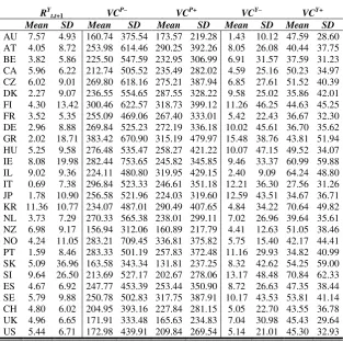
Summary statistics of vertex centralities and network centralization may be found in Tables 1 and 2. These statistics already reveal some asymmetric behaviour of co-movement of economic growth and stock markets. Compared to CP–-MST, average vertex centralities are usually higher for CP+-MST and compared to CY–-MST they are always higher for CY+-MST. It therefore seems that at least in average, markets and particularly economies tend to develop similarly when thriving. The effect is particularly strong for economic growth networks, where vertex centralities are much higher for positive growth then for negative. These results are confirmed by average network centralization as well. Note, that for networks of positive economic growth, the density is almost six times larger compared to networks of negative economic growth.

At first, these observations might seem to be contra-intuitive as it is widely believed, that during crisis periods, co-movement between markets (thus economies) should be higher. One would therefore expect that networks will be denser during periods of negative returns or negative growth. A more detailed analysis revealed that extreme densities are larger for networks constructed from negative returns/growth. For example, the highest centralization of stock market networks constructed from negative returns was 81.92 during the fourth quarter of 2008 (the peak of the financial crisis, e.g. the bankruptcy of Lehman Brothers). Highest centralization of stock market networks constructed from positive returns was only 26.26 during the second quarter of 2009 (recovery after the crisis). Although the differences were not that extreme, similar story is visible also from networks of real economic growth. It therefore seems that extreme declines occur jointly across stock markets and in lesser extent also across economies.

Table 1 Network variables: centralization

NCP– NCP+ NCY– NCY+

Mean 6558.13 6756.21 217.09 1260.87

SD 12859.22 7571.82 742.36 746.74

Table 2 Country specific variables: real economic growth and vertex’s centralities

RYt,t+1 VC

P–

VCP+ VCY– VCY+

Mean SD Mean SD Mean SD Mean SD Mean SD

AU 7.57 4.93 160.74 375.54 173.57 219.28 1.43 10.12 47.59 28.60 AT 4.05 8.72 253.98 614.46 290.25 392.26 8.05 26.08 40.44 37.75 BE 3.82 5.86 225.50 547.59 232.95 306.99 6.91 31.57 37.59 31.23 CA 5.96 6.22 212.74 505.52 235.49 282.02 4.59 25.16 50.23 34.97 CZ 6.02 9.01 269.80 618.16 275.21 387.94 6.85 27.61 51.52 40.39 DK 2.27 9.07 236.55 554.65 287.55 328.22 9.58 25.02 35.86 42.01 FI 4.30 13.42 300.46 622.57 318.73 399.12 11.26 46.25 44.63 45.25 FR 3.52 5.35 255.09 469.06 267.40 333.01 5.42 22.43 36.67 32.30 DE 2.96 8.88 269.84 525.23 272.19 336.18 10.02 45.61 36.70 35.62 GR 2.02 18.71 383.42 670.90 315.19 479.97 15.48 38.76 43.81 51.94 HU 5.25 9.58 276.48 535.47 258.27 421.22 10.07 47.15 49.52 34.07 IE 8.08 19.98 282.44 753.65 245.82 345.85 9.46 33.37 60.99 59.88 IL 9.02 9.36 224.11 480.80 319.95 429.15 2.40 9.09 64.24 48.80 IT 0.69 7.38 296.84 523.33 246.61 351.18 12.21 36.30 27.56 31.26 JP 1.78 10.90 256.58 521.96 224.03 319.60 12.59 43.51 34.67 36.71 KR 11.36 10.77 234.07 487.01 290.49 407.65 4.84 34.22 70.64 49.82 NL 3.73 7.29 270.33 565.38 238.01 299.11 7.02 26.96 39.64 35.61 NZ 6.98 9.17 156.94 312.06 160.89 217.79 4.41 12.63 51.05 38.46 NO 4.24 11.05 283.21 709.45 336.81 375.82 5.75 15.40 42.17 44.41 PT 1.59 8.46 283.33 501.19 257.83 372.48 11.16 29.93 34.82 40.99 SK 5.09 36.96 163.58 343.34 131.81 237.25 8.32 42.62 54.25 59.00 SI 9.64 26.50 213.69 527.17 202.67 278.06 13.17 48.48 70.84 62.33 ES 4.67 6.92 247.77 453.39 253.44 350.90 8.72 26.63 47.35 38.44 SE 5.79 9.88 250.78 502.83 317.75 387.91 10.17 43.53 53.81 41.14 CH 4.80 6.02 204.95 393.16 227.84 281.15 5.05 22.70 43.55 36.78 UK 4.96 6.65 171.91 333.48 165.63 234.83 7.04 30.98 45.43 29.64 US 5.44 6.71 172.98 439.91 209.84 269.54 5.14 21.01 45.30 32.93

Notes: All values were multiplied by 1000

With specification (8) we use centralities and centralization from networks constructed separately for positive and negative returns/growth. Our motivation for such approach was that an economy can have the same level of centrality regardless of whether the previous growth was positive or negative; the same applies for stock market networks

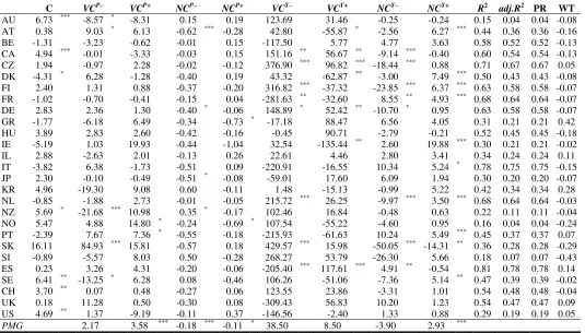
We can evaluate the whole panel of data, i.e. 68 quarterly observations across all countries using the pooled mean group estimator (PMG). The resulting coefficients can be interpreted as long-run coefficients (Pesaran and Smith, 1995). Our results show, that statistically significant are only centralizations of both stock market networks and networks of real economic growth.

Based on the result reported in Table 3, it seems, that isolating the centralities and centralization based on the sign of returns is really useful when forecasting future output. To highlight the most interesting results, we will focus on the PMG estimates.

whether the increased density of the stock market network was during bearish or bullish market conditions.

Finally, the disentanglement of the output growth networks shows that higher centralization of the output growth network is followed by higher level of output growth, if

network’s centralization is related to positive growth. This result shows that from forecaster’s

perspective, what really matters is whether economies have similar positive growth.

Table 3 Predicting next quarter’s change in real economic growth using vertex’s harmonic centrality and overall harmonic centralization of a network of positive or negative return co-exceedances

C VCP– VCP+ NCP– NCP+ VCY– VCY+ NCY– NCY+ R2 adj.R2 PR WT

AU 6.73 *** -8.57 * -8.31 0.15 0.19 123.69 31.46 -0.25 -0.24 0.15 0.04 0.04 -0.08 AT 0.38 9.03 * 6.13 -0.62 *** -0.28 42.80 -55.87 * -2.56 6.27 *** 0.44 0.36 0.36 -0.16 BE -1.31 -3.23 -0.62 -0.01 0.15 -117.50 5.77 4.77 3.63 0.58 0.52 0.52 -0.13 CA 4.94 *** -0.01 -3.33 -0.03 0.15 151.16 ** 56.67 ** -9.14 *** -0.40 0.60 0.54 0.54 -0.13 CZ 1.94 -0.97 2.28 -0.02 -0.12 376.90 *** 96.82 *** -18.44 *** 0.88 0.71 0.67 0.67 0.05 DK -4.31 * 6.28 -1.28 -0.40 0.19 43.32 -62.87 ** -3.00 7.49 *** 0.50 0.43 0.43 -0.08 FI 2.40 1.31 0.88 -0.37 -0.20 316.82 *** _{-37.32 -23.85} *** _6.37 *** _{0.63 0.58 0.58 -0.07} FR -1.02 -0.70 -0.41 -0.15 0.04 -281.63 ** -32.60 8.55 ** 4.93 *** 0.68 0.64 0.64 -0.07 DE 2.83 2.36 1.30 -0.40 * _{-0.06 148.89} * _52.42 ** _-10.70 * _{0.95 0.63 0.58 0.58 -0.07} GR -1.77 -6.18 6.49 -0.34 -0.73 * -17.18 88.47 6.56 4.05 0.31 0.21 0.21 0.42 HU 3.89 2.83 2.60 -0.42 -0.16 -0.45 90.71 -2.79 -0.21 0.52 0.45 0.45 -0.18 IE -5.19 1.03 19.93 -0.44 -1.04 32.54 -135.44 ** 2.60 19.88 *** 0.30 0.21 0.21 -0.02 IL 2.88 -2.63 2.01 -0.13 0.26 22.61 4.46 2.80 3.41 0.34 0.24 0.24 0.11 IT -3.82 6.38 -1.73 -0.51 0.09 -220.91 -16.55 10.34 5.24 * 0.78 0.75 0.75 -0.15 JP 2.30 -0.10 -0.49 -0.51 * -0.08 -59.01 17.60 6.09 1.94 0.30 0.20 0.20 -0.07 KR 4.96 -19.30 9.08 0.60 -0.11 1.48 -15.13 -0.99 5.22 0.42 0.34 0.34 0.28 NL -0.85 -1.88 2.73 -0.01 -0.05 215.72 *** 26.25 -9.97 *** 3.50 *** 0.68 0.64 0.64 -0.03 NZ 5.69 * -21.68 *** 10.98 0.35 * -0.17 102.46 16.84 -0.48 0.63 0.22 0.11 0.11 -0.04 NO 5.47 4.88 14.80 * -0.24 -0.69 * 107.54 -55.22 -4.60 0.95 0.16 0.04 0.04 -0.24 PT -2.39 7.67 7.36 * -0.55 -0.18 -215.93 -61.63 10.24 5.49 *** 0.45 0.37 0.37 0.07 SK 16.11 84.93 *** 15.81 -0.57 0.18 429.57 *** 15.98 -50.05 *** -14.31 ** 0.36 0.28 0.28 -0.29 SI -0.89 -5.57 8.03 0.50 -0.28 268.27 53.79 -26.30 5.66 0.18 0.07 0.07 -0.43 ES 0.23 3.26 4.31 -0.20 -0.06 -205.40 *** 117.61 *** 4.91 ** -0.54 0.81 0.78 0.78 0.14 SE 6.41 ** _-13.25 * _{6.28 0.08 -0.46 106.26 -51.06 -7.36 5.14} ** _{0.47 0.39 0.39 -0.02} CH 3.70 ** 0.07 0.48 -0.27 0.06 123.55 23.86 -3.31 1.01 0.54 0.48 0.48 -0.04 UK 0.18 11.28 0.50 -0.30 0.08 -309.43 56.83 10.20 1.23 0.54 0.47 0.47 0.09 US 4.69 ** 1.37 -9.19 -0.11 0.37 -146.56 -2.40 1.33 0.88 0.29 0.19 0.19 0.05 PMG 2.17 3.58 *** -0.18 *** -0.11 * 38.50 8.50 -3.90 2.93 ***

6. Conclusion

In this preliminary research note we provide empirical evidence, that stock market and output growth networks provide predictive in-sample power when explaining changes in the real output of 27 OECD economies over the years from 1998 to 2014. More specifically, for each time period, we construct networks based on stock market returns or the output growth. It is shown, that the topological properties of the resulting networks help to predict next quarter changes in the output of the economy.

References

1. Baur, D., Schulze, N. 2005. Coexceedances in financial markets—a quantile regression analysis of contagion. Emerging markets review, 6 (1), 21–43.

2. Billio, M., Getmansky, M., Lo, A. W., and Pelizzon, L. 2012. Econometric measures of

connectedness and systemic risk in the finance and insurance sectors. Journal of Financial Economics, 104 (3), 535–559.

3. Boldi, P., Vigna, S. 2014. Axioms of Centrality. Internet Mathematics, 10 (3-4), 222– 262.

4. Canova, F., De Nicolo, G. 1995. Stock returns and real activity: A structural approach.

European Economic Review, 39 (5), 981–1015.

5. Cribari-Neto, F. 2004. Asymptotic Inference under heteroscedasticity of unknown form.

Computational Statistics & Data Analysis, 45 (2), 215–233.

6. Cribari-Neto, F., Zarkos, S.G. 1999. Bootstrap methods for heteroskedastic regression models: evidence on estimation and testing. Econometric Reviews, 18 (2), 211–228.

7. Lin, J.W., McLeod, I. A. 2006. Improved Peňa–Rodriguez portmanteau test.

Computational Statistics & Data Analysis, 51(3), 1731–1738.

8. Mantegna, R. N. 1999. Hierarchical structure in financial markets. The European

Physical Journal B – Condensed Matter and Complex Systems, 11 (1), 193–197.

9. Newey, W. K., West, K. D. 1994. Automatic Lag Selection in Covariance Matrix

Estimation. The Review of Economic Studies, 61 (4), 631–653.

10. Peña, D., Rodríguez, J. 2006. The log of the determination of the autocorrelation matrix

for testing goodness of fit in time series. Journal of Statistical Planning and Inference, 136 (8), 2706–2718.

11. Pesaran, H.M., Smith, R. Estimating long-run relationships from dynamic heterogeneous

panels. Journal of Econometrics, 68 (1), 79–113.

12. Prim, R. C. 1957. Shortest connection networks and some generalizations. Bell System Technical Journal, 36 (6), 1389–1401.

13. White, H. 1980. A Heteroskedasticity-Consistent Covariance Matrix Estimator and a