The E Monetary Theory

Munich Personal RePEc Archive

The E-Monetary Theory

Ngotran, Duong

29 October 2016

Online at

https://mpra.ub.uni-muenchen.de/77206/

The E-Monetary Theory

∗

JOB MARKET PAPER

Duong Ngotran

First Version: Oct, 2016. This Version: Feb, 2017

University at Albany, State University of New York

Abstract

Using the sparse grid, we solve a DSGE model where there are two types of electronic money: reserves (e-money that is issued by the central bank for banks) and zero maturity deposits (e-money that is issued by banks). Transactions between bankers are settled by reserves, while transactions in the non-bank private sector are settled by zero maturity deposits. We use our model to discuss about unconventional monetary policy tools during the Great Recession. Due to the maturity mismatch between deposits and loans, we find that keeping the federal funds rate at the lower bound for a long but finite time stimulates the economy in the short run but creates deflation and lower outputs in the long run. To get out of the zero lower bound, the central bank can conduct helicopter money and increase the interest rate paid on reserves simultaneously, which is impossible in the Keynesian theory, but possible with the current electronic money system.

∗_{I would like to thank Adrian Masters for his guidance and support during this project. Special thanks to Daniel Betty,}

Michael Sattinger, Michael Jerison for helpful comments and discussions. I also thank to Jack Rossbach, John Jones, Yue Li, Ibrahim Gunay, Kajal Lahiri, Savita Ramaprasad, Minhee Kim, Garima Siwach, Kang Gusang, Tu Nguyen and other participants in workshops.

1

Introduction

Nowadays, money mostly exists in the electronic form. According to the data from the Federal Reserve

Bank, the total stock of M1 in Jun 2016 is around USD 3274 billion, consisting of USD 1381 billion in

currency and USD 1850 billion in checkable deposits. However, as the world currency, most US dollar bills

are held outside US. Judson (2012) estimates that 60 percent of US dollar bills are in foreign countries.

If we exclude that number from M1 and M2, currency only accounts for 15 percent of the M1 stock and

5 percent of the M2 stock. Moreover, the value of transactions conducted by currency is far less than the

ones with electronic money.Schreft and Smith(2000), based on the“Nilson Report 1997”, shows that cash accounts for 20 percent of the dollar volume of U.S. payments made by consumers in 1990 and 18 percent

in 1996, and is projected to account for only 16 percent in 2000 and 12 percent in 2005. In this paper, we

focus on a particular group of e-money issued by commercial banks, including checkable deposits, money

market deposit account and saving account. For convenience, we call this group as zero-maturity deposits

(ZMDs) thereafter.

ZMDs are different from currency in two salient features. First, in nature, currency is an IOU issued by

the central bank while ZMDs are IOUs issued by commercial banks. In economic terms, currency is outside

money while ZMDs are inside money. Second, unlike currency, ZMDs pay the (positive) nominal interest

rate. Banks pay the interest rate for saving account and money market deposits account for a long time, but

the tricky part is the checking account. In a frictionless perfectly competitive banking market, the interest

rate on checkable deposits should be positive and follow the federal funds rate. However, before 2012,

under the Regulation Q, banks in US were prohibited from paying interest on checking account. During

this period, banks still implicitly paid the demand deposit rate under the form of giving gifts or reducing

the cost of additional services to their customers, seeMitchell(1979),Startz(1979),Dotsey(1983). Becker

(1975) estimates that the implicit demand deposit rate in US during 1960-1968 was around 2.64

percent-3.74 percent.

Since 2012, the Regulation Q has been no longer valid, and most banks are now paying interest rate on

the checkable deposits (see Table8 in AppendixA). According to the data in September 2016 of Federal

Deposit Insurance Corporation (FDIC), the national average interest on checkable account is 0.04 percent,

on saving account is 0.06 percent. These rates are low as the federal funds rate is near zero. If the federal

the era of electronic money, it is more natural to model money as an interest-earning asset. Even during

the period of 2000-2012, as the popularity of credit cards and Internet banking helped people to conduct

transaction even with only saving account, it is more reasonable to model that households earn interest rate

from holding ZMDs.

This paper builds a dynamic general equilibrium model where currency does not exist. There are two

forms of money in our model: reserves and ZMDs. In our model, ZMDs are inside money issued by the

commercial banks. They are used for settling the transactions between every pair of agents in the economy,

except between bankers-bankers, bankers-government, and bankers-central bank. In these types of

transac-tions, bankers have to use reserves- another type of e-money that commercial banks deposit at the central

bank. Only government and commercial banks have an account at the central bank. The amount of ZMDs

banks can issue is restricted by two constraints: the reserves requirement and the capital requirement. In our

model, the central bank only controls the level of reserves while the level of money supply (total amount of

ZMDs) depends on the interaction between the central bank, the commercial banks and the public. In the

normal time when the reserves requirement is binding, by adjusting the level of reserves, the central bank

can target the interbank lending rate; and therefore the prime rate that banks lend out to households. In the

situation when the reserves requirement is not binding, the central bank can control the interbank lending

rate by adjusting the interest rate paid on reserves.

We use our theory to set lights on what happened in the Great Recession. Banks, in our model, hold an

asset related to the construction sector. When a big negative housing demand shock is realized, the price

of this asset drops. Bankers fire-sell this asset to satisfy the capital constraint, which further pushes down

its price. Consequently, bankers’ net worth decline to a new level that they need to cut loans to satisfy the

capital requirement constraint. The level of ZMDs declines even though the level of reserves go up. As

the price of loan is higher and the deflation episode is realized, the private investment declines strongly. If

the central bank only follows the conventional monetary policy where they purchase the small amount of

government bond from bankers to inject reserves, the recession will be severe. It takes a long time for the

loan market to be back into the normal mode.

Even though the only shock in our model comes from the households’ demand side, it does not affect the

household directly, but rather indirectly through the banking sector. When banks cut loans, the total amount

of money in the economy declines. As households need money in advance to purchase the final good and

Moreover, unlike the story in the collateral constraint1households want to sell house more quickly to relax

their liquidity constraint, which in turn, pushes down the housing price further and amplified the initial

housing demand shock.

We discuss in detail the unconventional monetary policy2when the central bank changes the component

of its balance sheet by purchasing the distressed assets rather than the government bonds. This program,

through the asset price channel, immediately pushes the commercial banks out of the capital constraint and

recover the credit flows between households and bankers. In the short run, this unconventional monetary

policy can prevent the prolonged deflation episode. However, in the medium run, without adjusting the

interest rate paid on reserves, deflation might happen as the result of keeping the interbank rate at the lower

bound for too long.

The intuition for the mechanism why deflation might happen in the medium run after the quantitative

easing (QE) can be explained by the mismatch between the maturity of money and loans in our model.

Bankers know that in the long run, the federal funds rate will be back to the steady state level, so when

making a long term loan, they have to take into account this effect into the current loan rate. If the central

bank keep the federal funds rate at the lower bound, the nominal deposit rate is also at the lower bound,

while the real loan rate might start rising if bankers know the rate will rise in the future. In equilibrium,

the real return on deposits will be equal to the real loan rate minus the liquidity premium. If the liquidity

premium does not change much, the deflation must realize to increase the real return on deposits to match

it up with the real loan rate.

The recommended policy for the central bank is to raise the interest rate paid on reserves on the exit

date from the zero lower bound, even if the central bank does not see the inflation signal. When the central

bank raises the federal funds rate, the deflation goes down further but it will pick up quickly as the nominal

interest rate on deposits start matching up with the real loan rate. To reduce the negative effect of temporary

rise in the federal funds rate, the Fed can use the helicopter money simultaneously. This policy is impossible

to conduct in the Keynesian theory, but is totally possible with the electronic money.

Our model can generate some key facts in the Great Recession: (i) the level of reserves skyrockets but

the money multiplier plummets, (ii) the interbank rate is equal to the interest rate paid on reserves for a 1_{If housing is in the collateral constraint, in the model without default, the price of housing will recover quickly as the shadow}

price of the collateral constraint pushes up the housing price

2_{In many contexts, it is called “quantitative easing” (QE) in our paper, even though our model does not examine the situation}

long time after the quantitative easing, (iii) the deleveraging process when banks actively cut loans, (iv)

the sharp cut of investment and outputs at the beginning of the housing crisis, (v) the sharp decline then

suddenly increase again of the inflation in only two quarters. Indeed, the last fact is the challenging to any

New Keynesian model to generate.

The are two main challenges in the computation method for our model. First, our model features the

three occasionally binding constraints, where the switch between reserves requirement and capital

require-ment play the key role. Second, our model has six state variables, one of which is the aggregate reserves

level. The level of reserves can be nearly five times as high as its steady state level in the simulation,

creat-ing the difficulty for buildcreat-ing a good grid. To conduct the quantitative exercise, we build a Smolyak grid in

Brumm and Scheidegger(2015) and use the nonlinear certainty equivalent (NLCEQ) approximation method

inCai, Judd and Steinbuks(2015) to estimate the decision rule. This global solution method is stable and

can handle three occasionally binding constraints in our model. For each point in the grid, NLCEQ uses it

as the initial state and transforms our stochastic problem into a deterministic problem. For large shock, to

solve the deterministic system, we also combine NLCEQ with the continuation method.

Related Literature

On the money supply side, our approach is similar toBianchi and Bigio(2014) andAfonso and Lagos

(2015) when the central bank can increase the level of money supply and cut down the federal funds rate

by injecting more reserves in the banking system. These papers explicitly model the search and matching

process of heterogeneous agents in the interbank market while the one in our model is frictionless with

identical bankers. In exchange of that, our model can connect the central bank policy to not only banks’

balance sheet but also the production sector, which is missing in bothBianchi and Bigio(2014) andAfonso

and Lagos(2015).

On the money demand side, our model follows the cash-in-advance literature. As our model does not

have currency, “cash” here should be interpreted as ZMDs. InBelongia and Ireland(2006,2014), currency

and deposits are bundled together and provide the liquidity service to households. Our deposits, however,

are zero maturity deposits. LikeLucas and Stokey(1987), households need money in advance to purchase

the consumption good. Even though money in our model earns the positive interest rate, its rate of return

is still less than the rate they borrow from bankers. We also extend the Clower constraint to the investment

and housing purchases (Stockman (1981), Abel (1985), Fuerst (1992), Wang and Wen (2006)). Indeed,

the income, rather than the consumption alone, to estimate the money demand function. The appearance

investment in the Clower constraint is important to generate the persistence of output and deflation.

We also share the sticky price feature with the New Keynesian framework. The important role of

finan-cial frictions in the New Keynesian has been emphasized for a long time (seeBernanke, Gertler and Gilchrist

(1999),Christiano, Motto and Rostagno(2004)). Recently, many New Keynesian research (Gertler and

Kiy-otaki(2010), Curdia and Woodford(2011), Gertler and Karadi (2011)) incorporates the banking sector to

their models, aiming to answer what happened in the Great Recession and the role of the unconventional

monetary policy, Our paper differs mainly from these line of research in the money supply process. We

can characterize the micro-foundation link between reserves, banks’ balance sheets, money supply and the

federal funds rate; hence, our model can exhibit the long duration of federal funds rate at the lower bound

after quantitative easing while this link is often missing in the New Keynesian literature. Moreover, the New

Keynesian often focuses on the interest rate channel, while the unconventional monetary policy in the Great

Recession inclines to the asset price channel and bank lending channel. Our model, somehow, can exhibit

all of those channels in a succinct framework.

Our approach also relates to a large literature in macro-finance where macro shocks can affect strongly

to the balance sheets of intermediaries. BothBrunnermeier and Sannikov(2016) and our model emphasize

the importance of inside money in the deflation episode. Both show the intermediaries cut the amount of

inside money they issue during the time their net worth decline, leading to the sharp decline in the money

multiplier during the crisis. However, two papers differ mainly in the role of money and the money supply

process. There is no reserves and two-tier money inBrunnermeier and Sannikov(2016). Moreover they

em-phasize the role of storing value in money while our paper focus on the function as the medium of exchange

in money. Gertler and Karadi(2011),He and Krishnamurthy(2013) andCaballero and Simsek(2013) also

show the circumstances when intermediaries fire sell their risky assets under the capital constraint, which is

2

The Environment

2.1

Notation:

LetPt be the price level (price of the final consumption good), we use the lower letter to exhibit the real

balance of a variable or its relative price. For example, the real reserves balancent=Nt/Pt, or the real price

ofpm_t =P_tm/Pt. The timing notation follows this rule: If a variable is determined or chosen at timet, it will

have the subscriptt. All of the interest rates in the model are gross nominal rates, except when explicitly stated differently. The gross inflation rate isπt =Pt/Pt−1.

2.2

Time, Demographics and Preferences

Time is discrete, indexed byt and continues forever. The economy has seven types of agents: bankers, households, wholesale firms, retail firms, construction firms, the government and the central bank.

There is a measure one of identical infinitely lived bankers in the economy. Bankers discount the future

with the rateβ. Each period, they gain utility from consuming the final consumption goodct. Their expected

utility at the periodtcan be written as:

Et " _∞

∑

βilog(ct+i) #

There is also a measure one of identical infinitely lived households. Households discount the future with

the rateβe<β, so they will borrow from the bankers. Each period, households gain utility from consuming

the final consumption goodct and enjoying the flow of housing service from the housing stockht. However,

they lose utility when providing laborelt to their own production. Household’s expected utility at the period

t can be written as:

Et " _∞

∑

e

βi log(c˜t+i) +ξtlog(h˜t+i)−χ

˜

l_t+i1+η

1+η

!#

whereξt is time-varying housing demand shock andηis the inverse Frisch elasticity of labor supply.

Wholesale firms, retail firms are infinitely lived, owned by households. Construction firms, like in

Gertler and Karadi(2011), finance their capital purchase by issuing a perfectly state-contingent securities

to bankers, so their profits are zero in every period.

collects tax from households to pay for the coupon for the outstanding government bonds (perpetuities).

The government is assumed to not issue new government bonds in our model.

The central bank uses the payoffs they get from holding the government bonds (or other assets) to pay

for the interest paid on reserves to bankers. The remaining payoffs are transferred back to the government

to transfer to households. The central bank also purchases or sells the government bonds to bankers every

period to adjust the level of reserves and the federal funds rate. In the unconventional monetary policy, the

central bank might purchase the financial claims on the construction firms from bankers.

2.3

Goods and Production Technology

There are four types of goods in the economy: final consumption goodyt produced by retailers, wholesale

goodsyt(j)produced by wholesale firm j, intermediate goodytmproduced by households, and housinght

produced by construction firms. Besides that, there are two types of capital in the economy:Kt andHt.

Each period households self-employ their laborelt and use the capitalKt−1to produce the homogeneous

intermediate goodym_t under the Cobb-Douglas production function:

ym_t =K_t−α₁el_t1−α

whereα is the share of capital in the production function. CapitalKdepreciates with the rateδ. Households also own a technology to convert one unit of final goodyt to one unit of capital typeK and vice versa. So

each period they also make an investmentIt. Households sellytmto wholesale firms.

There is a continuum of wholesale firms indexed by j ∈[0,1]. Each wholesale firm purchases the homogeneous intermediate goodym_t from households and differentiates it into a distinctive wholesale goods

yt(j)under the following technology:

yt(j) =ymt

Then retail firms produce the final goodyt by aggregating a variety of differentiated wholesale goods

yt(j):

yt =

Z 1

0

yt(j)

θ−1

θ _{d j}

θ

θ−1

Construction firms use the capitalHt−1 they purchase from other construction firms at the end of the

production function of a construction firm is:

ih_t =Ht−1

We assume that capital H is not depreciated and there is a total fixed amount H of this capital in the economy. In equilibrium,Ht=H. The stock of housing in the economy isht. Housing is depreciated with

the rateδh_{, so:}

ht = (1−δh)ht−1+iht

2.4

Asset Technology

There are four types of financial assets: government bondsbg_t, bank loansbh_t, financial claims on the con-struction firmsxt, and interbank loans btf. Let Pt be the price of the final goodyt, some of our financial

instruments are indexed to the price levelPt.

(a) Government bonds (bg_t): are issued by the government. They are traded between bankers and the

central bank. We assume that households do not hold government bonds. We model government bonds

bg_t as consols, which are indexed to the price levelPt. The owner of 1 unit of government bonds at time

twill receivePjunits of dollars for every period jwhere j≥t+1. The price of one unit of government

bond isqt. The total number of government bonds issued by the government is fixed.

(b) Bank loans to households (b_th): We follow Leland and Toft(1996) andBianchi and Bigio(2014) to

model the loan structure between bankers and households. We assume that the loan contract between

bankers and households is in a particular form that each period households only need to pay a fraction

δb of the total real debt stock in the previous periodbht−1. Letbht be the real loan stock in the periodt,

letst be the real flow of new loan issuance, we have:

bh_t = (1−δb)bht−1+st

In detail, the real flow new loans issuance st constitutes a promise from households to pay for the

bankers the nominal amountst(1−δb)nδbPt+1+n in periodt+n+1, for alln≥0. So banks’ loans are

also indexed to the price level. The price of loan rt is determined by a perfectly competitive market.

So if rt <1, bankers earn an immediate accounting profit (1−rt)st. Loans are illiquid and bankers

cannot sell loans.

(c) Financial claim on the construction firms (xt): are issued by the construction firms. We assume that

only bankers can purchase these claims as they have technology to verify the revenue of the construction

firms. It is also assumed that these claims can be traded between bankers. Each financial claim has a

pricevt and pays a stochastic real payoffrtx.

(d) Interbank loan (b_tf): Bankers can borrow reserves from other bankers in the federal funds market.

The nominal gross interest rate in the federal funds market is the federal funds rateR_tf.

2.5

Money

There are two types of electronic money in our economy: reservesnt and zero maturity depositsmt.

(a) Reserves (nt): is a type of e-money issued by the central bank. Only government and bankers have an

account at the central bank, so only government and bankers have reserves3. Each period, the central

bank pays a gross interest rate Rn on these reserves4. Reserves are used for settling the transactions between bankers and bankers, bankers and central bank, bankers and government.

(b) Zero maturity deposits (mt): is a type of e-money issued by the bankers. Each period, banks pay the

interest rateRm_t for these ZMDs which is determined by the perfectly competitive market. Moneymtis

used for settling the transaction in the private sector. These ZMDs are insured by the central bank, so

they are totally safe. ZMDs and reserves have the same unit of account.

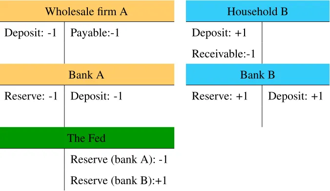
In the electronic payment system, there is a connection between the flows of reserves and deposits. For

example, we assume that wholesale firm A (whose account at bank A) pays 1 dollar for household B

(whose account at bank B). Then the flow of payment will follow Table (1). For a transaction between

government and households, or between the central bank and households, money still flows through banks,

so we can think this contains two sub-transactions. One is between government and banks, which is settled

by reserves. One is between banks and households, which is settled by ZMDs.

3_{The amount of US Treasury deposits at the Fed is not considered as reserves in reality. However, for convenience, we also}

call that money as reserves in our model. In equilibrium, the balance of the government account at the central bank is zero, so it does not matter.

4_{Throughout our paper, it is assumed thatR}n_{is a constant. Only in the section6.8, we considerR}n

t is a time-varying variable

Wholesale firm A Household B Deposit: -1 Payable:-1 Deposit: +1

Receivable:-1

Bank A Bank B

Reserve: -1 Deposit: -1 Reserve: +1 Deposit: +1

The Fed

Reserve (bank A): -1 Reserve (bank B):+1

Table 1: Electronic Payment System

2.6

Regulations

There are two central bank’s regulations that bankers have to face each period: reserves requirement and

capital requirement

(a) Reserves Requirement: At the end of each period, bankers have to hold enough reserves that is greater

or equal to a fractionϕ of total deposits.

(b) Capital Requirement: At the end of each period, bankers’ net worth must be greater or equal to a

fractionκ of the sum of their loan issuance and the total value of financial claims on the construction

firms.

2.7

Timing within one period

1. The housing demand shockξt realizes.

2. Production take places. Households produce the homogeneous intermediate goodsy_tmand sell them to wholesale producers . Wholesale producers differentiate them and sell to retailers. Retailers then

pro-duce the final consumption good. The construction firms also build new houses. All of the payments

of these transaction are delayed until the step 5.

4. The final good market and housing market open. Households need ZMDs in advance to purchase both

housing and final goods.

5. ZMD payments are settled: The retailers pay the wholesale firms. The wholesale firms pay

house-holds. The profits of wholesale firms are also distributed to househouse-holds. Tax/Transfer is sent from the

government to households. Payoffs from the financial claims on the construction firms go to bankers.

6. The banking market opens. Banker can adjust the level of reserves by borrowing in the interbank

market, receiving new deposits, trading xt or bgt with other bankers and central bank. The central

bank also pays the interest rate on reserves for bankers.

3

Agents’ Problems

3.1

Bankers

There is a measure one of identical bankers in the economy. These bankers have to maintain a good balance

sheet under the regulation of the central bank. There are five types of assets on the bankers’ balance sheet:

reserves (nt), government bonds (bgt), loans to households (bht), loan to other bankers (b f

t) and financial

claims on the construction firms (xt). The bankers’ liability side contains the zero-maturity deposits that

households deposit here (mt).

Banker

Reserves: nt Zero Maturity Deposits:

mt

R_tm

Govt bonds: b_tg×qt Net worth

Loans to households: bh_t

Claims on construction firms:xt×vt

Loans to other bankers: b

f t

R_tf

Cost: We assume that banks face two kinds of cost when issuing loan. First, it is the operating cost when

bankers have to manage to collect the payment from households on time. The operating cost, measured by

The second cost is an asymmetric adjustment cost when bankers change the size of loan stock:

f st bh_t−1

!

= υ

4max

(

st

bh_t−1−δb,0

)4

When households want to reduces their debt stock by borrowing less, banker incurs no cost. However, when

bankers want to increase the loan stock, they have to pay the marketing expense. These costs are in terms

of final goods. The parameterυ governs the size of this cost.

On the timing of the market, it is worth noting that bankers can adjust the level of their deposits and

reserves after households and firms pay for each other. When a wholesale firm, who has an account a bank

B, pays for a household, who has an account at bank A, the deposits and reserves of bank B will reduce by

the same amount, while the deposits and reserves of bank A will increase by the same amount. When the

different parties in the economy pay each other, a banker can witness the deposits and reserves outflow from

or inflow to his bank. LetNIFt be the net inflow of deposits and reserves go into their bank, bankers will

takeNIFt as given. When the banking market opens, as the deposit market is perfectly competitive, banker

can choose any amount ˆdt of deposit inflows or outflows to his bank. Hence, if we letdt=NIFt+dˆt, the

variabledt will be a choice variable in bankers’ problem.

In each period, bankers treat all the prices as exogenously and choose {ct,nt,bth,st,mt,b f

t,xt,dt,b g t} to

maximize their expected utility over a stream of consumptions:

maxEt " _∞

∑

βilog(ct+i) #

subject to

Rnnt−1

πt

+b_t−g ₁+b

f t−1

πt

+dt−Tt=nt+qt(bgt −b

g

t−1) +vt(xt−xt−1) +

b_tf

R_tf (Reserve Flows) (1) mt

Rm_t = mt−1

πt

+f st

bh_t−1

!

+νbh_t +rtst−δbbht−1+ct−xt−1rtx+dt−Tt (Deposit Flows) (2)

bh_t = (1−δb)bht−1+st (Loan Stocks) (3)

nt≥ϕ

mt

Rm_t (Reserves Requirement) (4)

nt+bgtqt+

b_tf R_tf +b

h

t +xtvt−

mt

R_tm ≥κ

bh_t +xtvt

Banker Banker Reserves: +dt Deposits: +dt Reserves: -(bgt −b

g t−1)qt

Bonds: +(bg_t −bg_t−1)qt

Table 2: Bankers choose more deposits (left) and purchase bonds (right)

The Fed Banker Households

Bank Reserves: -T Reserves: -T Deposits: -T Deposits: -T Tax Due: -T Treasury Deposit: +T

Table 3: Government collects tax from households

Banker Banker

Loans: +st Deposits: +rtst Loans: -δbbt−h 1 Deposits: -δbbht−1

Net worth: +(1−rt)st

Table 4: Banker issues loans (left) and collects loans (right)

Banker Banker

Deposits: +ct Deposits: +(f(.) +νbth)

Net worth: -ct Net worth: - (f(.) +νbht)

Table 5: Banker consumes (left) and pays for cost (right)

The equation (1) shows the evolution of reserves in the banker’s balance sheet. After receiving the

interest rate paid on reserves, the previous reserves balance becomesRnnt−1/πt. He also receives the payoffs

from holding government bondsbg_t−1; and collects the payment from the loan he lends out to other bankers in the previous period b_t−f ₁/πt. He can also increase his reserves by taking more depositsdt. When the

banker receives more deposit inflows, his reserves and his liability increase by the same amount (Table2).

That is the reason we seedt appear on both the equation (1) and (2). The similar effect can be found on

Tt- the net tax that the government imposes on households. In this case, bankers debit the households’

deposit accounts then transfer reserves from their accounts to the account of the government at the central

bank (Table3). Banker can then leave reservesnt at the central bank’s account to earn the interest rate, or

purchase the government bondsqt(bgt −b g

t−1), or purchase the financial claimsvt(xt−xt−1), or lend reserves

to another bankersb_tf/R_tf.

deposits (Table 4). So when they make a loan (rtst), the balance sheet expands. When they collect the

payoffs from the loan (δbbh_t−1), the balance sheet shrinks. The banker also issues their own deposits to

purchase the consumption good from firms (ct) and to pay the cost (in terms of final goods) related to lending

activities (f(st/bth) +νbth) (Table4). The total amount of deposits also decline when the construction firms

pay for the bankers (xt−1rxt).

Bankers face two constraints in every period. At the end of each period, banks have to hold enough

reserves as a fraction of total deposits (4). This constraint should be interpreted more broadly than the the

real life reserves requirement in US because the total ZMDs here include not only the checkable deposits

but also the saving account and money market deposit account.

The second constraint plays the key role in our model - the capital requirement constraint. The left

hand side of (5) is the banker’s net worth (capital), which is equal to total assets minus total liabilities. The

constraint requires bank to hold capital greater than a fraction of total loans they issue, where financial claim

is also considered as a type of commercial loans.

Let λt, µt be the Lagrangian multipliers attached to the reserves constraint and the capital constraint.

LetRx_t be gross nominal return on the financial claimxt, which is defined as:

Rx_t+1=(vt+1+r x

t+1)πt+1

vt

The first order conditions of the banker’s problem can be written as:

1

ct

=βR_tfEt

1

ct+1πt+1

+µt (6)

1

ct

=βR_tmEt

1

ct+1πt+1

+µt+ϕλt (7)

1

ct

=βEt

_Rx

t+1

ct+1πt+1

+ (1−κ)µt (8)

1

ct

=βRnEt

1

ct+1πt+1

+λt+µt (9)

1

ct

=βEt

1+qt+1

qtct+1

+µt (10)

holding reserves is the federal funds rate that bankers can earn when lending out reserves to other bankers.

From the equation (6) and (9), when the reserves requirement is no longer bound,R_tf =Rn.

We denote f_t′= f′(st/b_t−h ₁)and f_t+′ ₁= f′(st+1/bht). The first order condition for choosing the loan stock

can be written as:

1

ct

ν+rt+

f_t′ bh_t−1

!

=Et

β δb

ct+1

+Et

_βs

t+1ft+′ 1

ct+1(bht)2

+Et

"

β(1−δb)(rt+1bht + ft+′ 1)

ct+1bht

#

+ (1−κ)µt (11)

The price of loans that households borrow from bankersrtdepends onµt- the shadow price of the capital

constraint,ν- the monitoring cost and the adjustment cost. When the capital constraint is binding,rtis lower

than before, implying that the real cost of borrowing for households increase.

3.2

Households/Intermediate Good Producers

There is a measure one of identical households. These self-employed households produce the homogeneous

intermediate goodymto sell to the wholesale firms atP_tm, or the real relative pricep_tm. In each period, house-hold purchases the final consumption good (_ect) from the retail firms and housing (eht) from the construction

firms. They also have a technology to convert one unit of consumption goods to one unit of capital type

K and vice versa . We assume the discount factor of the households is smaller than the discount factor of the bankers, βe(1+ν)<β, therefore, households will borrow from the bankers. Letebh_t be the debt stock that households borrow from bankers. Recalling from the section2.4, each period households only pay a

fractionδb of the old debts. We impose an exogenous borrowing constraint for households with the debt

limitbh_.

Households face the “ZMD-in-advance” when the good market opens. Let at be the amount of total

ZMDs that they hold when entering the goods market and housing market. Their total purchase of final

goods and new housing has to be less than or equal toat.

In each period, households choose{_ect,m_et,at,eht,elt,ebth,set,It,Kt,eiht}to maximize their expected utility:

maxEt "

∞

∑

e

βi log(c˜t+i) +ξtlog(h˜t+i)−χ

˜

l_t+i1+η

1+η

subject to

at+δbebt−h 1= e

mt−1

πt

+rtset (Loans Market Open) (12)

e

ct+It+qtheiht ≤at (ZMDs-in-advance) (13) e

mt

Rm_t +cet+δbeb

h

t−1+qtheiht +It+Tt =

˜

mt−1

πt

+rtset+ptmymt +

Π_t

Pt

(Budget Constraint) (14)

eih_t =eht−(1−δh)h˜t−1 (Residential Investment) (15)

It=Kt−(1−δ)Kt−1 (Investment) (16)

e

bh_t = (1−δb)ebt−h 1+est (Loan Stock) (17)

ym_t =K_t−α₁el_t1−α (Production Function) (18)

e

bh_t ≤bh _{(Borrowing Constraint) (19)}

The equation (12) shows the constraint households face when the loan market opens but the final good

market has not opened yet. Households bringm_et/πt amount of money from the previous period, obtaining

new loanrtest, paying back a fraction of the previous loan δbebht−1, and bringat amount of money into the

final good market.

The constraint (13) is the “cash-in-advance” constraint inLucas and Stokey(1987). The only difference

here is that currency does not exist in our model, so “cash” should be interpreted as ZMDs. Households

need ZMDs in advance to purchase the consumption goods, housing and making investment. Wang and

Wen(2006) shows that putting investment in the cash-in-advance constraint can generate the persistence of

output and inflation in the data.

The equation (14) shows the typical budget constraint households face in each period. After paying

the debts (δbebh_t−1) in the previous period to the banker, and obtaining new loans (rtest), in addition to their

previous balance in the deposit account ( ˜mt−1/πt), households will receive income from selling

intermedi-ate goods (pm_t ym_t ) and the profits from the wholesale firms (Π_t). They spend on consumption goods (_ect),

investmentIt, new housingeith, leave some money as the zero-maturity deposits at the banksmet/Rmt , and pay

(receive) the tax (transfer)Tt to the government.

The equation (18) shows the production function of households. In each period, households combine

their own labor and capital in the Cobb-Douglas form to produce the intermediate goods. Here we assume

hire labor in the competitive market.

We assume that households face an exogenous borrowing constraint, rather than a collateral borrowing

constraint like Kiyotaki and Moore (1997) and Iacoviello (2005). Our purpose is to emphasize that the

mechanism of the shock transmission in our model is not related to the collateral constraint literature.

We model housing as a durable good. Housing is depreciated at the rateδh_{. There is a housing demand}

shock in our model, captured by the time-varying parameter ξt. We assume the motion of ξt follows the

equation:

log(ξt) = (1−ρ)log(ξ) +ρlog(ξt−1) +εt, εt∼N(0,σ2) (20)

Letγt,Λ_t,ωt be respectively as the Lagrangian multiplier for the constraint (13), (14) and (19). We have:

1

e

ct

−γt−Λt=0 (21)

Λ_t =βeRm_t Et

1

e

ct+1πt+1

(22)

qh_t

e

ct = ξ_˜t

ht

+βe(1−δh)Et "

qh_t+1

e

ct+1

#

(23)

χel_tη+1= (1−α)Λ_tpm_t y_tm (24)

rt e

ct

=β δe bEt

1

e

ct+1

+βe(1−δb)Et

rt+1

e

ct+1

+ωt (25)

1

e

ct

=βe(1−δ)Et

1

e

ct+1

+βeEt

_αΛ

t+1pmt+1ymt+1

Kt

(26)

From the equations (21) and (22), we can rewrite:

1

e

ct

=βeRm_t Et

1

e

ct+1πt+1

+ γt

| {z }

Liquidity Premium

As money plays the role of medium of exchange in our model, it’s value contains the liquidity part. In

the steady state, the rate of return on money has to be less than 1/βe- the risk-free rate that households lend

out to each other (if possible). This equation plays the important role when we analyze the implication when

the central bank keeps the interest rate at the lower boundRnfor a long time.

The equation (25) gives us the marginal cost and the marginal benefit when households borrow one

can relax both cash-in-advance constraint and the general budget constraint, allowing the households to

consume more. The left hand side of (25) is the marginal benefit when household borrow one more unit of

st with the pricert. The marginal cost is more challenging to understand as the maturity of loan is not finite.

When households borrow one more unit ofst, in the next period, they have to payβ δe bst, so it explains the

first part on the right hand side of the equation (25). The second part is the present value of the remaining

debts carrying on to the following period after households borrow one more unit ofst. The final component

is the shadow priceωt of the borrowing constraint. In our model, the borrowing constraint will be bound at

the steady state. However, the interesting part of our paper happens when bankers actively cut the level of

loans and the constraint (19) is no longer binding,ωt=0.

Similarly, the marginal cost and the marginal benefit when household invest one more unit of capital

are showed in the equation (26). When households decide to transform 1 unit of consumption good to 1

unit of capital, the marginal cost (left hand side) is the marginal utility lost from not consuming this 1 unit.

However, if investing into capital, households receive two benefits in the next period. The first thing is

capital, after depreciation, can transform back to the consumption good for consuming in the future. The

second thing is the increase in the level of output in the next period from investing 1 more unit of capital in

this period.

3.3

Construction Firms

Competitive construction firms build houses that are eventually sold to households. At the end of the period

t, a construction firm acquires the capital Ht for use in the production in the subsequent period. It is noted

that the capital typeHis totally different from the capital typeK, and they are not substitutable. We assume capitalH is the only factor in the production function of construction firms. After production in the period

t+1, capital is not depreciated and the firm can sell the capital in the open market to other construction firms. There are no adjustment costs at the firm level, so the firm’s capital choice problem is always static.

The construction firms finance their capital acquisition in each period by obtaining funds from bankers.

FollowGertler and Karadi(2011), to acquire the funds to purchase capital at the end oft, the firm issuesxt

claims equal to the number of units of capital they acquireHt. Under the no arbitrage condition, the price

of each claimvt will be equal to the price of a unit of capital typeH.

It is assumed that the bankers has perfect information about the firm and has no problem enforcing

construction firms will always get zero profits, while the bankers might earn positive or negative profits

depended on the realization of the housing demand shock.

The production function of the construction firms is:

ih_t =Ht−1 (27)

Letqh_t be the price of houses in the periodt. Given that the construction firm earns the zero profit state-by-state,rx_t- the real payoffs (excluding the capital gain) paid to the owner of one financial claim-andRx_t - the gross nominal return for holding this claim- will be:

r_tx=q_th (28)

R_tx= (q h

txt+vtxt)πt

vt−1xt−1

(29)

3.4

Retail Firms

Retail firms competitively produce the final consumption goods. The retail firm buy and aggregate a variety

of differentiated wholesale goods indexed by j∈[0,1]using a CES technology:

yt =

Z 1

0 yt(j)

θ−1

θ _{d j}

θ

θ−1

whereθ is the elasticity of substitution among the wholesale goods. Profit maximization and the zero profit

condition give the demand for the wholesale good j

yt(j) =

Pt(j)

Pt

−θ

yt (30)

3.5

Wholesale Firms

There is a unit mass of wholesale firms on[0,1]that are monopolistic competitors. Wholesale firms buy the

intermediate goodym_t atP_tmfrom the households in a competitive market, differentiate the good at no cost intoyt(j)and sell it with the pricePt(j)to the retailer.

Follow Rotemberg pricing, we assume that each wholesale goods firm j faces costs of adjusting prices, which are measured in terms of final good and given by:

ι

2

Pt(j)

Pt−1(j)

−1

2

yt

whereιis the adjustment cost parameter which determines the degree of nominal price rigidity. The

whole-sale firm j discounts the profit in the future with rateβei_Λt+i/Λ

t, whereΛt is the shadow price attached to

the households’ budget constraint. The problem of firm jis given by:

max

{Pt(j)}

Et ∞

∑

βiΛt+i

Λt

"

Pt+i(j)

Pt+i

−pm_t+i

yt+i(j)−ι

2

Pt(j)

Pt−1(j)

−1

2

yt+j #)

subject to its demand in equation (30).

In a symmetric equilibrium, all firms will choose the same price and produce the same quantityPt(j) =Pt

andyt(j) =yt=ymt . The optimal pricing rule then implies that:

1−ι(πt−1) +ιβeEt

_Λ

t+1

Λ_t (πt+1−1)πt+1

yt+1

yt

= (1−p_tm)θ (32)

3.6

The Central Bank

The central bank conducts open market operation, by purchasing and selling government bonds with bankers

every period, to target the the interest rate R_tf that bankers borrow from each other. By purchasing the government bonds held by bankers, it increases the level of reserves, relaxing the reserves requirement

constraint, and therefore lowering the federal funds rate and the prime rate.

When we model explicitly the process of how the central bank controls the federal funds rate, the

“traditional” Taylor rule is not enough for the determinacy. There are infinite levels of reserves that satisfy

R_tf =Rn. Hence, when the federal funds rate is at its lower bound, we need a rule governing the motion of the level of reserves (reserves targeting) (Figure1).

We assume that the central bank follows the hybrid rule which is resulted from the combination of federal

funds rate targeting and reserves targeting:

R_tf =Rf_+φ n

nt−(1−ρn)n−ρnnt−1

n

Demand   Supply  

Reserves   Discount  Rate  

IROR   FFR  

Before  Great   Recession  

A<er  GR  

Figure 1: The Federal Funds Market

whereρnis the persistence of the level of reserves;φn,φπ andφyis the coefficient responding to the reserve

gap, inflation gap and output gap;Rf_{,n,π andyare the federal funds rate, reserves, inflation and final good}

outputs at the deterministic steady state.

Like the Taylor rule in the New Keynesian literature, the interbank rate responds to the output gap

and the inflation rate. However, this rule departs from the traditional Taylor rule in two important points.

First, it also includes the gap between the current level of reserves and its steady state value. The return

of the federal funds rate to the steady state value is not enough to guarantee that the level of reserves and

government bonds held by bankers also back to the steady state. Therefore, the federal funds rate should

respond to the reserves gap. Does the appearance of reserves gap change significantly the Taylor rule?

The answer is no, φn is positive but very small so it nearly does not have any effects when the reserves

requirement is still binding.

Second, unlike the conventional Taylor rule, we do not see the zero lower bound here. This is one of the

most interesting points in our model. The natural lower bound for the federal funds rate in our model is the

interest rate paid on reserves. When the central bank injects the amount of reserves over the critical point

from targeting the federal funds rate to targeting the level of reserves to responds to the output gap and the

inflation rate. It also implies that when the banking system is awash of reserves, the central bank can still

control the federal funds rate by changing its policy on interest rate paid on reserves. We will discuss this

policy later in the paper. For now, we assumeRn is constant and the central bank will only follow the rule in (33).

3.7

The Government

We assume the government is totally independent from the central bank. It does not change its fiscal policy

in our model. The total outstanding government bonds is fixed. Each period, the government collects tax

from households to pay coupons for the government bond holders, which are central bank and bankers.

When the central bank receives the payoffs from government bonds, they use them to pay the interest

rate paid on reserves for bankers (Rn−1)nt−1/π. We assume that central bank holds a big number of

government bonds such that the payoffs are greater than (Rn−1)nt−1/π. After that, for the remaining

payoffs, the central bank will transfer them back to the government, who in turn will transfer it back to

households. So letTt be the net tax households (in real term) have to pay:

Tt=bg_t−1+

(Rn−1)nt−1

πt

(34)

It is worth noting that, as government bonds are indexed, we do not have to keep track the balance sheet of

the Fed explicitly. It is no longer true if we assume the central bank holds nominal long term government

bond.

4

Equilibrium

Definition: A competitive equilibrium is a stochastic sequence of bankers’ decision choice{ct,nt,bh_t,st,mt,

b_tf,xt,dt,bg_t}, household’s choice {_ect,ebth,set,met,elt,Kt,It,yemt }, wholesale firm’s choice {ytm}, retail firm’s

choice{yt}, the government tax {Tt}, and the market price {rt,Rtf,qt,πt,pmt }such that given the market

The market clearing condition implies that:

Net flows of reserves between bankers: dt=0 (35)

The interbank market: b_tf =0 (36)

Total ZMDs: mt=met (37)

Loan Market: bh_t =eb_th (38)

Capital H and Financial claim: xt=Ht =H (39)

Housing Market: ieh

t =ith=H (40)

Consumption Good Market: yt=ct+cet+It+νbht +f

st

bh_t−1

!

+ι

2(πt−1)

2_y

t (41)

It is worth noting that, as the reserves only flow from one bank to another bank, the total net flows of

reserves in equilibrium will be zero. If we only consider the symmetric competitive equilibrium where all

banks are identical, then dt must be zero. This condition, (34), (36) and (39) imply that the evolution of

reserves (1) in the banking system, in equilibrium, can be written as:

nt−1

π =nt+qt(b

g

t −b

g t−1)

In the conventional monetary policy, we assume that the central bank only purchase the government

bonds. Under that condition, the level of reserves in the banking system will increase when the central bank

conducts the open market purchase and reduce when they conducts the open market sales. It is emphasized

here that the level of reserves in the banking system is decided solely by the central bank. Each individual

commercial bank can change its own level of reserves, but the sum amount of reserves are not decided by

commercial banks. Under the normal condition, by manipulating the level of reserves, the central bank can

adjust the federal funds rate and the level of money supply.

The right hand side of the equation (41) shows the aggregate demand of the economy. We can

decom-pose it into four components: (i) the aggregate consumption as the sum of bankers’ consumption (ct) and

households’ consumption (_ect), (ii) the private investment (It), (iii) the cost of providing services in the

bank-ing sector νbh

t +f(.)and (iv) the inflation cost. When the housing demand shock ξt is realized, later we

will see that the decline inIt is the biggest factor for the collapse of the aggregate demand.

5

The Deterministic Steady State

To ensure that in the steady state, households will borrow from banker and the borrowing constraint is

binding, we assume that the discount rate of households is smaller than the one of bankers after adjusting

for the cost of loan.

Assumption 1:

e

β(ν+1)<β

Assumption 2:

The long-run interbank rate that the central bank target is1/β.

Rf _{=1/β >R}n

Theorem 1: Under the Assumption (1) and (2), the deterministic steady state where Rf _{=1/β will lie in}

the region where the capital constraint is slack (µ =0) and the reserves constraint is binding (λ >0).

From the Assumption 2 and (6), ifµ>0 thenRf _{<1/β, lower than the central bank long run target. If}

λ =0, thenRf _=Rn_{, which is contradict with the Assumption 2. We want to restrict ourself to the steady}

state similar to the banking state before the Great Recession to illustrate the effect of housing crisis on the

economy.

6

Quantitative Analysis

6.1

Calibration

We calibrate the banker’s discount factor β =0.99, implying the federal funds rate at the steady state is

around 4.04 percent annually, which is roughly matched with the average of the effective federal funds

rate before the Great Recession. The reserves requirementϕ and nare set to match the ratio between the amount of zero maturity deposits and the level of reserves in the banking system. ZMDs are calculated as

the difference between the total MZM (money zero maturity) and the currency. We average the ratio data

between ZMDs and reserves during the 2008Q1, which is around 527 times, orϕ=0.199. For the capital

parameterν is set to make the bank’s loan rate to household is around 0.5 percent higher than the federal

funds rate in the steady state. The fraction of paid loan δb is set to 0.2, which is 20 percent of the total

loan stock. It is important to remark here that our banker’s balance sheet does not contain the time deposit

(both small-denomination and large denomination), which accounts for approximately 25 percent of total

bankers’ asset.

For the households, the parameters { βe, χ, η, δ, α } are calibrated in the standard way. The two

nonstandard parameters are ξ, the relative utility weight of housing, and bh_{, the exogenous borrowing}

constraints. We calibrateξ so the total value of financial claims on the construction firms accounts for 35

percent of total banker’s asset. We should interpret that these financial claims also account partial to the level

of mortgage loans in the commercial bank’s balance sheet. So more than one third of commercial banks’

balance sheet in our model is exposed to the housing demand shock. The other nonstandard parameter is

bh, which is set so the total household debt is around 100 percent of household’s consumption.

On the supply side, we calibrate the elasticity of substitution between wholesale goods is 4, which is in

range from 3 to 5, that is common in the literature. The cost of changing price in the Rotemberg model is

set to 50.

About the central bank’s rule, the reaction of the federal funds rate to the output gap is set to 0.25/4, to

the inflation gap is set to 1.5. A new parameter appears in our model isρn, the persistence in the level of

reserves. We set it at the level of 0.8, means that once the Fed injects a lot of reserves in the banking system,

the central bank will not drain it quickly in the following period. We can say that the flow of reserves is

smooth.

6.2

Solution Method

We focus on the recursive competitive equilibrium when the prices and decision rules are the functions of

state variables. Our problem has 6 state variables{bg_t−1,nt−1,mt−1,bht−1,Kt−1,ξt}when we assume the

cen-tral bank follows the conventional monetary policy by purchasing only government bonds. The problem has

3 occasionally binding constraints, which are the reserves requirement constraint, the capital constraint and

the borrowing constraint. These constraints require us to use a global solution to solve the model. Moreover,

some variables, like reserves and the amount of government bonds held by bankers, can jump to points very

far from the steady state. Reserves can be five times as high as the level at the steady state. As the result

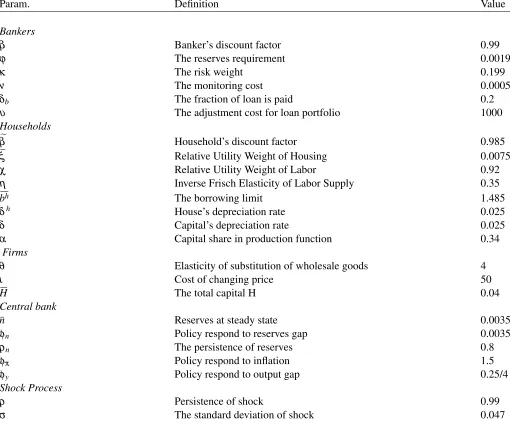
Table 6: Parameter values

Param. Definition Value

Bankers

β Banker’s discount factor 0.99

ϕ The reserves requirement 0.0019

κ The risk weight 0.199

ν The monitoring cost 0.0005

δb The fraction of loan is paid 0.2

υ The adjustment cost for loan portfolio 1000

Households e

β Household’s discount factor 0.985

ξ Relative Utility Weight of Housing 0.0075

χ Relative Utility Weight of Labor 0.92

η Inverse Frisch Elasticity of Labor Supply 0.35

bh _{The borrowing limit 1.485}

δh _{House’s depreciation rate 0.025}

δ Capital’s depreciation rate 0.025

α Capital share in production function 0.34

Firms

θ Elasticity of substitution of wholesale goods 4

ι Cost of changing price 50

H The total capital H 0.04

Central bank

n Reserves at steady state 0.0035

φn Policy respond to reserves gap 0.0035

ρn The persistence of reserves 0.8

φπ Policy respond to inflation 1.5

φy Policy respond to output gap 0.25/4

Shock Process

ρ Persistence of shock 0.99

σ The standard deviation of shock 0.047

approximation method inCai, Judd and Steinbuks(2015) to solve our model. This method contains three

main steps: (i) build a grid and transform a stochastic problem into a deterministic problem, (ii) solve the

deterministic problem in each grid point to find the next period decision’s rule, (iii) finally approximate the

decision rule in whole grid from the results in step 2. The method is global and deals well with the inequality

constraint. However, we will lose some accuracy from ignoring the uncertainty when agents make decision.

In this paper, we use the software Ipopt (Interior Point Method) written byWachter and Biegler(2006) to

solve the large system of equation in each grid point.

points to refine the grid adaptively. The description of how to build this grid is presented in the Appendix

(B). Smolyak grid can deal with the “curse of dimensionality” problem in macroeconomics. It detail

de-scription and applications in economics can be found in Malin, Krueger and Kubler (2011), Judd et al.

(2014), Brumm and Scheidegger (2015). In our problem, when building grid, we also use the adaptive

domain technique inJudd et al.(2014) for the two pairs of state variablesbg-n, andbh-m. When the central bank conducts the open market purchase, the increase of reserves nt is associated with the decrease the

government bond held by banker. It is likely that we are never in a state that both reserves and government

bonds held by banker are at the high level, so for these two states, we put them in a parallelogram rather

than a rectangular. The same principle is applied forbh and mas they tend to move together in the same direction. Judd et al.(2014) use the stochastic simulation from the solution of linear model to identify the

adaptive domain region while we only use the ad-hoc way to identify the adaptive domain.

For each grid point (each initial state), we solve the deterministic problem, and assume that after T=500,

the economy will be back to the steady state. To deal with the inequality constraints, we use the penalty

method found inMcGrattan (1996) to transform the hard constraint into soft constraint. We assume the

utility in one period of bankers has the form:

u(ct,λt∗,µt∗) =log(ct)−

1

4emax{λ

∗ t ,0}4−

1

4emax{µ

∗ t,0}4

λ_t∗= mt

Rm_t − nt

ϕ

µ_t∗= mt

R_tm−

h

nt+qtbgt + (1−κ)(bth+xtvt) i

wheree=1e8 is the penalty coefficient. It means that any time, bankers violate the reserves requirement constraint or the capital constraint, they suffer the reduction in their utility. However, if they hold more

reserves or capital than the required amount, they are not rewarded for that. This penalty method is also

applied for the households’ borrowing constraint. Cash-in-advance constraint is always binding in the

deterministic model, so we do not need to transform it.

This setup still ensures that all of our first order conditions are twice differentiable. However, even

with this transformation, our system of equations is still ill-conditioning. Most of the time, we have to use

the homotopy method in combination with nonlinear large scale optimization tool Ipopt to solve the big

6.3

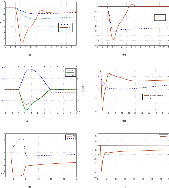
Housing Crisis and Conventional Monetary Policy

6.3.1 Shock Transmission in Interbank Market

When a big negative shock on housing demandξt is realized, price of housingqht drops. Consequently, the

pricevt of the financial claimsxt on the construction firms and bankers’ net worth must go down. In the

conventional monetary policy, the central bank will conduct the open market purchase to push down the

interbank rate R_tf. As the price is sticky, the real rate will go down, pushing up the price of government bonds and other assets. This can mitigate the initial decline invt and bring the economy back to the normal

state.

However, when the shock is large and persistent, the conventional monetary policy is not enough for

controlling the decline invt, especially when the capital constraint is bound. The decline ofvt pushes down

the banker’s capital. If bankers’ net worth goes down to the level where the capital constraint is binding,

bankers have to relax this constraint by reducing the loan sizebhand the number of financial claims on the construction firms xt on their balance sheets. This fire sales create the negative externalities as it further

pushes down thevt and bankers’ net worth.

To see the whole process clearly, we start from the equation (28) and impose the equilibrium condition

xt =H:

R_tx= (q h

t +vt)πt

v_t−1

The above equation decomposes the return on the financial claim into two components: the real payoffqh_t

and the capital gain when reselling these financial instrumentvt. When substituting it into (8), we have:

vt

ct

=βEt

"

qh_t+1+vt+1

ct+1

#

+ (1−κ)µt (42)

Solving this Euler equation forward and impose the transversality condition, the price vt of the financial

claimxtis:

vt=Et " _∞

∑

ct+j

qh_t+j

#

+ (1−κ)Et

" _∞

∑

ct+j

µt+j #

(43)

Similarly, we can solve forward for the priceqt of government bonds from (10):

qt =Et " _∞

∑

ct+j #

+Et

" _∞

∑

ct+j

µt+j #

From (43) and (44), we can express the pricevt as the function of government bond’s price, the discounted

housing price from future and the discounted of the shadow price of capital constraint:

vt = qt |{z}

Govt bonds’ price

+Et

" _∞

∑

βj

ct

ct+j

(qh_t+j−1)

#

| {z }

Adjusted discounted house prices

−κEt

" _∞

∑

βj

ct

ct+j

µt+j #

| {z }

Shadow price of capital constraint

(45)

The conventional monetary policy can push up the price of government bonds; and therefore, increasing

the price of other assets. However, with a big housing demand shock, the decline of the second term

outweighs the increase in the first term. When the capital constraint starts binding, the contribution of the

increase in the shadow price of capital constraint declinesvt further. Even when the central bank pushesRtf

to its lower bound (the interest rate paid on reservesRn