Munich Personal RePEc Archive
Sovereign Defaults and Banking Crises
Sosa-Padilla, Cesar
University of Notre Dame
August 2017
Online at
https://mpra.ub.uni-muenchen.de/81795/
Sovereign Defaults and Banking Crises
IC´esar Sosa-Padilla
University of Notre Dame
Abstract
Episodes of sovereign default feature three key empirical regularities in connection with the
banking systems of the countries where they occur: (i) sovereign defaults and banking crises
tend to happen together, (ii) commercial banks have substantial holdings of government debt,
and (iii) sovereign defaults result in major contractions in bank credit and production. This
paper provides a rationale for these phenomena by extending the traditional sovereign default
framework to incorporate bankers who lend to both the government and the corporate sector.
When these bankers are highly exposed to government debt, a default triggers a banking
cri-sis, which leads to a corporate credit collapse and subsequently to an output decline. When
calibrated to the 2001-02 Argentine default episode, the model is able to produce default in
equilibrium at observed frequencies, and when defaults occur credit contracts sharply,
gener-ating output drops of 7 percentage points, on average. Moreover, the model matches several
moments of the data on macroeconomic aggregates, sovereign borrowing, and fiscal policy. The
framework presented can also be useful for studying the optimality of fractional defaults.
Keywords: Sovereign Default, Banking Crisis, Credit Crunch, Endogenous Cost of Default,
Bank Exposure to Sovereign Debt.
JEL: F34, E62
II thank Ricardo Reis (editor) and two anonymous referees for valuable comments and insights. For guidance
and encouragement, I thank Pablo D’Erasmo, Enrique Mendoza, and Carmen Reinhart. I have also benefited from comments and suggestions by ´Arp´ad ´Abrah´am, Qingqing Cao, Rafael Dix-Carneiro, Aitor Erce Dominguez, Juan Carlos Hatchondo, Daniel Hernaiz, Leonardo Martinez, Doug Pearce, Mike Pries, John Rust, Juan Sanchez, Eric Sims, Nikolai Stahler, Carlos Vegh, and seminar participants at U. of Maryland, Univ. Nac. de Tucum´an, EPGE - FGV, McMaster U., NCSU, UTDT, U. of Western Ontario, York U., U. of Toronto, U. de Montreal, EUI, Notre Dame, UCSC, GWU, Bank of England, FRB Atlanta, FRB Richmond, FRB St. Louis, IADB Research, the 2011 SCE–CEF Conference, the 2013 CEA Annual Meeting, the 2014 SED Conference, and the 2015 RIDGE Sov. Debt Workshop. Matt Brown, Shahed K. Khan and Niu Yuanhao provided excellent research assistance. All remaining errors are mine.
1. Introduction
1
Sovereign defaults and banking crises have been recurrent events in emerging economies.
2
Recent default episodes in emerging economies (e.g., Russia 1998, Argentina 2001-02) have
3
shown that whenever the sovereign decides to default on its debt there is an adverse impact on
4
the domestic economy, largely through disruptions of the domestic financial systems. Why does
5
this happen? Both in the Argentine and Russian cases (and also in others discussed below),
6
the banking sectors were highly exposed to government debt. In this way a government default
7
directly decreased the value of the banking sector’s assets. This forced banks to reduce credit to
8
the domestic economy (acredit crunch), which in turn generated a decline in economic activity.
9
The recent debt crisis in Europe also highlights the relationship between defaults, banking
10
crises, and economic activity. In early 2012, most of the concerns around Greece’s possible
11
default (or unfavorable restructuring) were related to the level of exposure that banks in Greece
12
and other European countries had to Greek debt. The concerns were not only about losing what
13
had been invested in Greek bonds, but also, and mostly, over how this shock to banks’ assets
14
would impact their lending ability and ultimately the economic activity as a whole.1
15
This leads to the realization that sovereign default episodes can no longer be understood
16
as events in which the defaulter suffers mainly from international financial exclusion and trade
17
punishments. The motivation above, the empirical evidence reviewed later on, and the policy
18
discussions (e.g., IMF, 2002, Lane, 2012) all suggest shifting the attention to domestic financial
19
sectors and how they channel the adverse effects of a default through the rest of the economy.
20
The main contribution of this paper is in the quantification of the impact that a sovereign
21
default has on the domestic banks balance sheets, their lending ability and economy-wide
22
activity. To do so, we build on the work of Brutti (2011), Sandleris (2016), and Gennaioli et al.
23
(2014) to apply a theory of the transmission mechanism of sovereign defaults to a quantitative
24
setup. We endogenize the output cost of defaults in the following way: a sovereign default
25
1
triggers a credit crunch, and this credit crunch generates output declines. Ours is the first
26
quantitative paper to endogenize the output cost of default as a function of the repudiated
27
debt. This makes our framework a natural starting point to study the optimality of fractional
28
defaults.
29
Based on three key empirical regularities, namely that (i) defaults and banking crises tend
30
to happen together, (ii) banks are highly exposed to government debt, and (iii) crisis episodes
31
are costly in terms of credit and output, we build a theoretical framework that links defaults,
32
banking sector performance, and economic activity. This paper rationalizes these phenomena
33
extending a traditional sovereign default framework (in the spirit of Eaton and Gersovitz, 1981)
34
to include bankers who lend to both the government and the corporate sector. When these
35
bankers are highly exposed to government debt, a default triggers a banking crisis which leads
36
to a corporate credit collapse and consequently to an output decline.
37
These dynamics that characterize a default and a banking crisis are obtained as the optimal
38
response of a benevolent planner: faced with a level of spending that needs to be financed,
39
and having only two instruments at hand (debt and taxes), the planner may find it optimal
40
to default on its debt even at the expense of decreased output and consumption. The planner
41
balances the costs and benefits of a default: the benefit is the lower taxation needed to finance
42
spending, and the cost is the reduced credit availability and the subsequently decreased output.
43
Quantitative analysis of a version of the model calibrated to the 2001-02 Argentine default
44
yields the following main findings: (1) default on equilibrium, (2) v-shaped behavior of output
45
and credit around crisis episodes, (3) mean output decline in default episodes of approximately
46
7 percentage points, and (4) the overall quantitative performance of the model is in line with
47
the business cycle regularities observed in Argentina and other emerging economies.
48
Layout. The remainder of this section reviews the related literature and the empirical evidence
49
motivating the paper. Section 2 introduces the economic problem of banks with holdings of
50
defaultable government debt. Section 3 describes the rest of the model economy and defines the
51
equilibrium. Section 4 presents details of the calibration and the numerical solution. Section
52
5 has the main results, and Section 6 presents robustness exercises. Section 7 concludes. All
53
tables and graphs are at the end of the manuscript.
1.1. Related literature
55
This paper belongs to the quantitative literature on sovereign debt and default, following the
56
contributions of Eaton and Gersovitz (1981) and Arellano (2008). In particular, a related work
57
is by Mendoza and Yue (2012) who are the first to endogenize the cost of default: a sovereign
58
default forces the private sector to use less efficient resources. We propose an alternative and
59
complementary source for output costs: a disruption in domestic lending triggered by
non-60
performing sovereign bonds in domestic banks’ balance sheets.
61
In recent years there has been a surge in studies looking at the feedback loop between
62
sovereign risk and bank risk. Acharya et al. (2014) model a stylized economy where bank
63
bailouts (financed via a combination of increased taxation and increased debt issuance) can solve
64
an underinvestment problem in the financial sector, but exacerbate another underinvestment
65
problem in the non-financial sector. Higher debt needed to finance bailouts dilutes the value of
66
previously issued debt, increases sovereign risk and creates a feedback loop between bank risk
67
and sovereign risk because banks hold government debt in their portfolios. On the policy side,
68
Brunnermeier et al. (2011) argue for the creation of European Safe Bonds as a way to break
69
this feedback loop. The idea relies on pooling (buying debt from all the European countries)
70
and tranching (securitization of those bonds into two tranches: a small and safe senior tranche,
71
and a larger and riskier junior tranche). Regulatory reform will in turn induce banks to hold
72
the senior tranche breaking the link between sovereign risk and bank risk.
73
Other researchers have recently (and independently) noticed the link between sovereign risk
74
and bank fragility, and have studied how it affects borrowing policies and default incentives.
75
Gennaioli et al. (2014) construct a stylized model of domestic and external sovereign debt in
76
which domestic debt weakens the balance sheets of banks. This potential damage to the
bank-77
ing sector represents in itself a signaling device that attracts more and cheaper foreign lending.
78
Balloch (2016) studies an economy where domestic banks demand government debt for its
79
colateralizability properties (above and beyond its financial return). Domestic bank holdings
80
serve as an imperfect commitment device, and help the sovereign to raise funds from abroad
81
at lower rates.2 Our analysis relates to these papers in that it also identifies the damage that
82
2
financial institutions suffer during defaults. We identify the reduced credit as the endogenous
83
mechanism generating output costs of defaults and also analyze the benefit side: how
distor-84
tionary taxation can be reduced when defaults occur. Additionally, our dynamic stochastic
85
general equilibrium model allows us to quantify the importance of the “balance-sheet channel”
86
while also being able to account for various empirical regularities in emerging economies. 3
87
Recent work has also study the effects of banks’ exposure and default risk on the domestic
88
economy. Broner et al. (2014) provide a model with creditor discrimination and financial
fric-89
tions, where an increase in sovereign risk incentivizes domestic holdings of sovereign debt (due
90
to discrimination in favor of domestic creditors), crowds-out private investment and generates
91
an output decline. Bocola (2016) studies the macroeconomic implications of increased sovereign
92
risk in a model where banks are exposed to government debt. His framework takes default risk
93
as given and shows how the anticipation of a default can be recessionary on its own. Perez
94
(2015) who also studies the output costs of default when domestic banks hold government debt.
95
Public debt serves two roles in his framework: it facilitates international borrowing, and it
pro-96
vides liquidity to domestic banks. We relate to these studies in analyzing the balance-sheet
97
effects of a sovereign default in a quantitative model where default decisions are endogenous.
98
Finally, this paper also relates to recent research on optimal fiscal policy in the presence
99
of sovereign risk. Pouzo and Presno (2016) study the optimal taxation problem of a planner
100
in a closed economy with defaultable debt. Our main differences with Pouzo and Presno
101
(2016) are two: firstly, they rely on an exogenous cost of default, whereas we propose an
102
endogenous structure; and secondly, they assume commitment to a certain tax schedule but
103
not to a repayment policy, whereas we assume no commitment on the part of the government.
104
Kirchner and van Wijnbergen (2016) study the effectiveness of debt-financed fiscal stimulus
105
when government debt is held by leveraged-constrained domestic banks. Higher government
106
deficits tighten banks’ leverage constraint and create a crowding-out effect on private investment
107
(which may offset the initial stimulus). We also analyze the dynamic relationship between
108
government policy and bank holdings of sovereign debt, but our focus is on the default incentives
109
and output costs rather than on the stabilizing effects of government stimuli.
110
3
1.2. Empirical evidence
111
In this sub-section we review the three main empirical regularities that motivate this study.
112
Defaults and banking crises tend to happen together. A recent empirical study on banking crises
113
and sovereign defaults is the one by Balteanu et al. (2011). Using the dates of sovereign debt
114
crises provided by Standard & Poor’s and the systemic banking crises identified in Laeven and
115
Valencia (2008), they build a sample with 121 sovereign defaults and 131 banking crises for 117
116
emerging and developing countries from 1975 to 2007. Among these, they identify 36 “twin
117
crises” (defaults and banking crises): in 19 of them a sovereign default preceded the banking
118
crisis and in 17 the reverse was true. 4
119
Banks are highly exposed to sovereign debt. Kumhof and Tanner (2005) define the “exposure
120
ratio” of a given country as the financial institutions’ net credit to the government divided by
121
the financial institutions’ net total assets. Using IMF data for the period 1998-2002 they report
122
an average exposure ratio of 22% for all countries, 24% for developing economies, and 16% for
123
advanced economies. Interestingly, for countries that actually defaulted this ratio was even
124
higher (e.g., Argentina: 33%, Russia: 39%). A more recent empirical study by Gennaioli et al.
125
(2016) reports an average exposure ratio of 9.3% when using granular data from Bankscope
126
(which includes banks from both advanced and developing countries). When they focus only
127
on defaulting countries, they find an exposure ratio of roughly 15%. 5
128
Crisis episodes are characterized by decreased output and credit. It has been documented that
129
output falls sharply in the event of a sovereign default. The estimates vary across the empirical
130
literature, but all show that the output costs of defaults are sizable (e.g., Reinhart and Rogoff,
131
2009 report an 8% cumulative output decline in the three-year run-up to a domestic and external
132
default crisis). 6 Additionally, output exhibits a v-shaped behavior around defaults.
133
These crises are also characterized by decreased credit to the private sector. Data from the
134
Financial Structure Dataset (Beck et al., 2010) indicate that private credit (as a percentage of
135
GDP) falls on average 8% in the default year and remains low for the subsequent periods.
136
4
Previous empirical studies have found similar results, e.g. Borensztein and Panizza (2009) and Reinhart and Rogoff (2009), among many others.
5
Broner et al. (2014) also document the increase in exposure experienced in European countries since 2007.
6
2. Modeling bankers
137
The quantitative impact of sovereign defaults and banking crises depends on the specifics
138
of the transmission mechanism. This mechanism, in turn, depends on the modeling of the
139
financial sector, and so we devote this section to the bankers’ problem describing the market
140
for loanable funds and discussing the main assumptions. The rest of the model economy, which
141
is standard in the quantitative literature of sovereign debt, is presented in the next section.
142
2.1. Preliminaries
143
Bankers are assumed to be risk-neutral agents. In each period, they participate in two
144
different credit markets: the loan market (between private non-financial firms and bankers)
145
and the sovereign bond market (between the domestic government and bankers). The working
146
assumption is that they participate in these markets sequentially. 7
147
The bankers lend to both firms and government from a pool of funds available to them
148
during each period. These bankers start the period with the following resources: A, s(k) and
149
b. A represents an exogenous endowment, which the bankers receive each period. 8 s(k) is
150
the return on a storage technology: the previous period the banker put k into this technology,
151
and today the return is s(k). b represents the level of sovereign debt owned by the bankers at
152
the beginning of the period (which was optimally chosen in the previous period). Hereinafter
153
d2 {0,1} will stand for the default policy, with d= 1 (0) meaning default (repayment).
154
Sequence of events for the bankers. Firstly, the banker receives the endowment,A, has access to
155
the stored funds from the previous period, s(k), and gets government debt repayment, b(1−d).
156
Secondly, with those funds in hand, the banker extends intraperiod loans to firms, ls. Finally,
157
at the end of the period, the banker collects the proceeds from the loans, ls(1 +r), and then
158
solves a portfolio problem: chooses how much to lend to the government, (1−d)qb0, and how
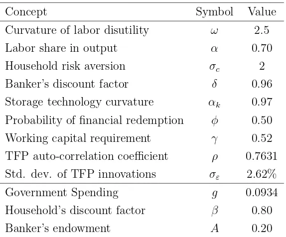
159
much to store, k0, with the remainder being left for consumption, x.
160
7
The assumption of sequential banking is no different from the day-market/night-market assumption com-monly used in the money-search literature (e.g., Lagos and Wright, 2005).
8
2.2. Bankers problem
161
From the above timing we have that lending to the firms is limited by the funds obtained at
162
the beginning of the period: F ≡A+s(k) +b(1−d). This is captured in the following lending
163
constraint: ls ≤ F. The problem of the bankers can be written in recursive form as:
164
W(b, k, z) = max
{x,ls,b0,k0
} !
x+δEW(b0, k0, z0) "
(1)
s.t. x = F +lsr−k0−(1−d)qb0 (2)
ls ≤ F (3)
F ≡ A+s(k) +b(1−d) (4)
where W(·) is the banker’s value function, E is the expectation operator, b0 represents
165
government bonds demand, q is the price per sovereign bond, r is the interest rate on the
166
private loans, x is the end-of-period consumption of the banker (akin to dividends), δ stands
167
for the discount factor, and z is the aggregate productivity. We can rewrite (1) - (4) as follows:
168
W(b, k;z) = max
{ls,b0,k0,µ
} !
A+s(k) +b(1−d) +lsr−k0−(1−d)qb0
+δEW(b0, k0;z0) +µ[A+s(k) +b(1−d)−ls]
" .
Assuming differentiability of W(·), the first-order conditions are:
169
ls : r−µ= 0 (5)
k0 : −1 +δE{Wk0}= 0 (6)
b0 : −(1−d)q+δE{Wb0}= 0 (7)
µ : A+s(k) +b(1−d)−ls ≥0 & µ[A+s(k) +b(1−d)−ls] = 0 (8)
Combining equations (5), (6), and the envelope condition with respect to k, we obtain:
which defines the optimal choice of k0. Combining equation (7) with the envelope condition
170
with respect to b we obtain:
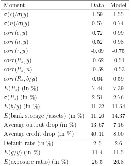
171
q=
8 <
:
δE{(1−d0)(1 +r0)} if d= 0
0 if d= 1 (10)
This expression shows that in the case of a default in the next period, (d0 = 1) the lender
172
loses not only its original investment in sovereign bonds but also the future gains that those
173
bonds would have created had they been repaid. These gains are captured by r0.
174
Equation (10) is the condition pinning down the price of debt subject to default risk in
175
this model. It is similar to the one typically found in models of sovereign default with
risk-176
neutral foreign lenders, where δ is replaced by the (inverse of the) world’s risk-free rate, which
177
represents the lenders’ opportunity cost of funds.
178
The loan supply function (ls) is given by:
179
ls=
8 <
:
A+s(k) + (1−d)b if r≥0
0 if r <0
(11)
2.3. Loan market characterization
180
A central aim of this model is to highlight how a sovereign default generates a credit crunch,
181
which translates into an increase in borrowing costs for the corporate sector (firms) and a
182
subsequent economic slowdown. This mechanism puts the financial sector in the spotlight and
183
Figure 1 shows how the private credit market reacts to a sovereign default. The supply for
184
loans was just derived above, the demand for loans comes from the problem of firms (detailed
185
in the next section) and responds to standard working capital needs.
186
Given that the intraperiod working capital loan is always risk-free (because firms are
as-187
sumed to never default on the loans), the bankers will supply inelastically the maximum amount
188
that they can. This inelastic supply curve is affected by a default: when the government
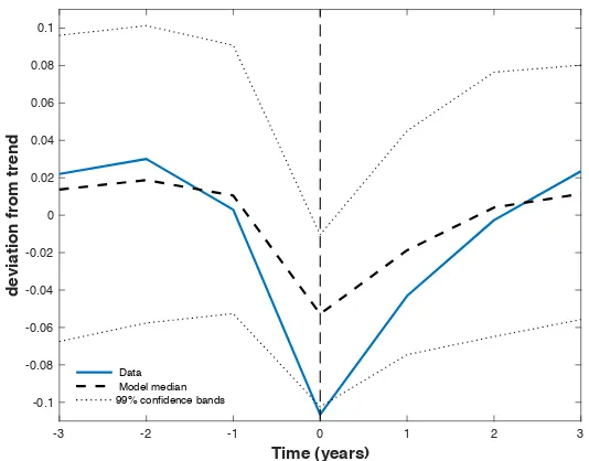
de-189
faults, bankers’ holdings of government debt become non-performing and thus cannot be used
190
in the private credit market. This is graphed as a shift to left of the ls curve in Figure 1. This
191
ends up in firms facing higher borrowing costs (r∗
d=1 > rd∗=0) and getting lower private credit in
192
equilibrium. The planner (whose problem is defined in section 3.4) takes into account how a
193
default will disrupt this market.
2.4. Discussion of the main assumptions
195
Absence of deposits. The main simplifying assumption in the modeling of bankers is having no
196
deposits dynamic. Instead, we assume that they receive a constant flow every period: this allows
197
us to fix ideas and focus on the asset side of the bankers’ balance sheet and how it responds
198
to a sovereign default. Incorporating deposits can make the effects of a default even larger:
199
(i) following the logic of Gertler and Kiyotaki (2010) (also used in Balloch, 2016), modeling
200
deposits we could have bankers as leveraged-constrained agents and so receiving a negative
201
wealth shock (like a sovereign default) will force them to decrease their liabilities (deposits),
202
which will in turn constrain even further the supply of loanable funds and make the effect of
203
a default even stronger; and (ii) anticipating the possibility of a sovereign default and fearing
204
that bankers will not be able to fully repay deposits, households may engage in a run on the
205
bankers, and thus put more contractionary pressure on the supply of loanable funds.
206
Both these effects go in the same direction and so our results can be understood as a lower
207
bound for the effects of sovereign defaults on the domestic supply of credit. Hence, we see the
208
absence of deposits as a sensible modeling assumption given that: (i) it renders the problem
209
more tractable and the dimensionality of the state space smaller, and (ii) it is conservative on
210
the quantitative impact of our mechanism.
211
Constant A. Even when abstracting from deposits may be convenient for computational
pur-212
poses, assuming a constant A may be unnecessarily simplistic from a calibration point of view.
213
In section 6.2 we relax this assumption and instead model the endowmentAas a function of the
214
general state of the economy (i.e. as a function of aggregate productivity). This modification
215
allows for procyclical flows to banks (a feature of the data) and makes defaults even tougher
216
on the domestic economy: when times are bad (low productivity), a default shrinks the supply
217
of domestic credit even more. 9
218
No foreign lenders. Another simplifying assumption is that the private sector can only borrow
219
from domestic lenders. Allowing the private sector to borrow also from abroad will decrease
220
the relevance of the domestic credit market for domestic production and potentially weaken the
221
channel highlighted in the model. However, as long as a fraction of the domestic firms need to
222
9
borrow from domestic sources (probably because not every firm in the economy is capable of
223
tapping international markets), the mechanism proposed in the model will still play a central
224
role in our understanding of the dynamics of macroeconomic aggregates and the incentives to
225
default on sovereign debt. Moreover, this assumption has robust empirical support as the vast
226
majority of corporate credit in emerging economies comes from domestic bank lending. 10
227
3. (Rest of the) Model economy
228
Time is discrete and goes on forever. There are four players in this economy: households,
229
firms, bankers (whose problem was already outlined in Section 2), and the government. In
230
this framework, the households do not have any inter-temporal choice, so they make only two
231
decisions: how much to consume and how much to work. The production in the economy is
232
conducted by standard neoclassical firms that face only a working capital constraint: they have
233
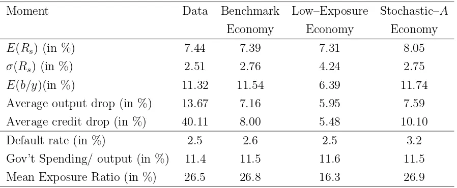
to pay a fraction of their wage bill up-front which creates a need for external financing.
234
The bankers lend to both firms and government, and also have access to a storage technology.
235
Finally, the government is a benevolent one (i.e., it maximizes the households’ utility). It faces
236
a stream of spending that must be financed and it has three instruments for this purpose:
237
labor income taxation, borrowing, and default. We assume the government has no commitment
238
technology, and this means that in each period it can default on its debt. This default decision is
239
taken at the beginning of the period and it influences all other economic decisions. Accordingly,
240
the following subsections examine how the economy works under both default and no-default,
241
and ultimately how the sovereign optimally chooses its tax, debt, and default policies.
242
3.1. Timing of events
243
If the government starts period t in good credit standing (i.e., not excluded from the credit
244
market), the timing of events is as follows (whereprimed variables represent next-period values):
245
- Period t starts and the government makes the default decision: d 2 {0,1}
246
1. if default is chosen (d = 1) then:
247
10
(a) the government gets excluded and the credit market consists of only the
(in-248
traperiod) private loan market: firms borrow to meet the working capital
con-249
straint and bankers lend (ls) up to the sum of their endowment and stored funds
250
(A+s(k)).
251
(b) firms hire labor, produce and then distribute profits (ΠF) and repay principal
252
plus interest of the loan (ls(1 +r)).
253
(c) bankers choose how much to store for next period (k0).
254
(d) labor and goods markets clear, and taxation (τ) and consumption take place.
255
(e) at the end of period-t a re-access coin is tossed: with probabilityφ the
govern-256
ment will re-access in the next period with a ‘fresh start’ (i.e., with b0 = 0), and
257
with probability 1−φ the government will remain excluded in the next period.
258
2. if repayment is chosen (d= 0) then:
259
(a) the credit market now consists of two markets: the one for working capital loans
260
and the one for government bonds. The bankers serve first the working capital
261
market (ls) up to the sum of their endowment, stored funds and the repaid
262
government debt (A+s(k) +b).
263
(b) firms hire labor, produce and then distribute profits (ΠF) and repay principal
264
plus interest of the loan (ls(1 +r)).
265
(c) bankers decide on sovereign lending (qb0) and storage (k0).
266
(d) labor and goods markets clear, and taxation and consumption take place.
267
- Period t+1 arrives
268
3.2. Decision problems
269
Here we describe the decision problems of households and firms, and also state the
govern-270
ment budget constraint.
271
Households’ problem. The only decisions of the households are the labor supply and
consump-272
tion levels. Therefore, the problem faced by the households can be expressed as:
273
max
{ct,nt}10 E
0
1 X
t=0
βtU(ct, nt) (12)
where U(c, n) is the period utility function, ct stands for consumption, nt denotes labor
274
supply,wtis the wage rate,τt is the labor-income tax rate, and ΠFt represents the firms’ profits.
275
Solving the problem we obtain:
276
−Un
Uc
= (1−τt)wt, (14)
which is the usual intra-temporal optimality condition equating the marginal rate of
substi-277
tution between leisure and consumption to the after-tax wage rate. Therefore, the optimality
278
conditions from the households’ problem are equations (13) and (14).
279
Firms’ problem. The firms demand labor to produce the consumption good. They face a
280
working capital constraint that requires them to pay up-front a certain fraction of the wage
281
bill, which they do with intra-period loans from bankers. Hence, the problem is:
282
max
{Nt,ldt}
ΠF
t = ztF(Nt)−wtNt+ldt −(1 +rt)ldt (15)
s.t. γwtNt ≤ ltd (16)
where z is aggregate productivity, F(N) is the production function, ld
t is the demand for
283
working capital loans,rt is the interest rate charged for these loans, andγ is the fraction of the
284
wage bill that must be paid up-front.
285
Equation (16) is the working capital constraint. This equation will always hold with equality
286
because firms do not need loans for anything else but paying γwtNt; thus any borrowing over
287
and above γwtNt would be sub-optimal. Taking this into account we obtain the following
288
first-order condition:
289
ztFN(Nt) = (1 +γrt)wt, (17)
which equates the marginal product of labor to the marginal cost of hiring labor once the
290
financing cost is factored in. Therefore, the optimality conditions from the firms’ problem are
291
represented by equation (17) and equation (16), evaluated with equality.
292
Government Budget Constraint. The government has access to labor income taxation and (in
293
case it is not excluded from credit markets) debt issuance in order to finance a stream of public
spending and (in case it has not defaulted) debt obligations. Its flow budget constraint is:
295
g + (1−dt)Bt =τtwtnt+ (1−dt)Bt+1qt (18)
where Btstands for debt (with positive values meaning higher indebtedness),g is an
exoge-296
nous level of public spending, and τtwtnt is the labor-income tax revenue.
297
3.3. Competitive Equilibrium given Government Policies
298
Definition 1. A Competitive Equilibrium given Government Policies is a sequence of
alloca-299
tions {ct, xt, nt, Nt, ldt, lst, kt+1, bt+1}1t=0 and prices {rt, wt,ΠFt}1t=0, such that given sovereign bond
300
prices {qt}1t=0, government policies {τt, dt, Bt+1}1t=0, shocks {g, zt}1t=0, and initial values k0, b0,
301
the following holds:
302
1. {ct, nt}1t=0 solve the households’ problem in (12) - (13).
303
2. {Nt, ltd}1t=0 solve the firms’ problem in (15) - (16).
304
3. {xt, lts, kt+1, bt+1}1t=0 solve the bankers’ problem in (1) - (3).
305
4. Markets clear: nt=Nt, bt =Bt, ldt =lst; and
306
the aggregate resources constraint holds: ct+xt+kt+1+g =ztF(nt) +A+s(kt).
307
3.4. Determination of Government Policies
308
We focus on Markov-perfect equilibria in which government policies are functions of
payoff-309
relevant state variables: the level of public debt, the level of storage held by bankers and
310
aggregate productivity. The benevolent planner wants to maximize the welfare of the
house-311
holds. To do so it has three policy tools: taxation, debt, and default. But it is subject to two
312
constraints: (1) the allocations that emerge from the government policies should represent a
313
competitive equilibrium, and (2) the government budget constraint must hold.
314
The government’s optimization problem can be written recursively as:
315
V(b, k, z) = max
d2{0,1} '
(1−d)Vnd(b, k, z) +d Vd(k, z)( (19)
where Vnd (Vd) is the value of repaying (defaulting). The value of no-default is:
316
Vnd(b, k, z) = max
{c,x,n,k0,b0}{U(c, n) +βEV(b
0, k0, z0)} (20)
subject to:
g+b=τ wn+b0q (gov’t b.c.)
c+x+g+k0 =zF(n) +A+s(k) (resources const.)
x= (A+s(k) +b)(1 +r)−k0−qb0
q =δE{(1−d0)(1 +r0)}
1 = sk(k0)δE{1 +r0}
r = znFn
A+s(k)+b − 1 γ
−Un
Uc = (1−τ)w
w= zFn
(1+γr)
9 > > > > > > > > > > > > = > > > > > > > > > > > > ;
(comp. eq. conditions)
318
The value of default is:
319
Vd(k, z) = max {c,x,n,k0
} '
U(c, n) +βE-φV(0, k0, z0) + (1−φ)Vd(k0, z0).( (21)
subject to:
320
g =τ wn (gov’t b.c.)
c+x+g+k0 =zF(n) +A+s(k) (resources const.)
x= (A+s(k))(1 +r)−k0
1 = sk(k0)δE{1 +r0}
r= znFn
A+s(k) − 1 γ
−Un
Uc = (1−τ)w
w= zFn
(1+γr)
9 > > > > > > > > > = > > > > > > > > > ;
(comp. eq. conditions)
321
3.4.1. Recursive Competitive Equilibrium
322
Definition 2. The Markov-perfect Equilibrium for this economy is (i) a borrowing ruleb0(b, k, z),
323
and a default rule d(b, k, z) with associated value functions {V(b, k, z), Vnd(b, k, z), Vd(k, z)},
324
consumption, labor and storage rules{c(b, k, z), x(b, k, z), n(b, k, z), k0(b, k, z)}, and taxation rule
325
τ(b, k, z), and (ii) an equilibrium pricing function for the sovereign bond q(b0, k, z), such that:
326
1. Given the price q(b0, k, z), the borrowing and default rules solve the sovereign’s
maximiza-327
tion problem in (19) – (21).
328
2. Given the price q(b0, k, z) and the borrowing and default rules, the consumption, labor
329
and storage plans{c(b, k, z), x(b, k, z), n(b, k, z), k0(b, k, z)}are consistent with competitive
330
equilibrium.
3. Given the price q(b0, k, z) and the borrowing and default rules, the taxation rule τ(b, k, z)
332
satisfies the government budget constraint.
333
4. The equilibrium price function satisfies equation (10)
334
4. Numerical Solution
335
We solve the model using value function iteration with a discrete state space. 11 We solve
336
for the equilibrium of the finite-horizon version of our economy, and we increase the number
337
of periods of the finite-horizon economy until value functions and bond prices for the first and
338
second periods of this economy are sufficiently close. We then use the first-period equilibrium
339
objects as the infinite-horizon-economy equilibrium objects.
340
4.1. Functional Forms and Stochastic Processes
341
The period utility function of the households is:
342
U(c, n) =
/
c−nω
! 01−σc
1−σc
(22)
where σc controls the degree of risk aversion and ! governs the wage elasticity of the labor
343
supply. These preferences (called GHH after Greenwood et al., 1988) have frequently been
344
used in the Small Open Economy - Real Business Cycle literature (e.g. Mendoza, 1991). This
345
functional form turns off the wealth effect on labor supply and thus helps in avoiding the
346
potentially undesirable effect of having a counter-factual increase of output in default periods.12
347
The bankers’ storage technology is:
348
s(k) =kαk
. (23)
The production function available to the firms is:
349
F(N) = Nα. (24)
11
The algorithm computes and iterates on two value functions: Vnd
andVd
. Convergence in the equilibrium price functionqis also assured.
12
The only source of exogenous uncertainty in this economy is zt, total factor productivity
350
(TFP). The logarithm of TFP follows an AR(1) process:
351
log(zt) =ρlog(zt−1) +"t (25)
where "t is an i.i.d. N(0, σ"2).
352
4.2. Calibration
353
The model is calibrated to an annual frequency using data for Argentina from the period
354
1980-2005. Table 1 contains the parameter values.
355
The parameters above the line are either set to independently match moments from the
356
data or are parameters that take common values in the literature. The labor share in output
357
(α) and the risk aversion parameter for the households (σc) are set to 0.7 and 2 respectively,
358
which are standard values in the quantitative macroeconomics literature. The working capital
359
requirement parameter (γ) is taken directly from the Argentine data. In the model γ is equal
360
to the ratio of private credit to wage payments and the data show that for Argentina this ratio
361
was 52%. 13 We use TFP estimates from the ARKLEMS team in order to estimate ρ and σ ".
362
The discount factor for the bankers (δ) takes a usual value in RBC models with an annual
363
frequency, 0.96. It is important to realize that the exact value of δ is crucial not in itself but
364
in how it compares with the households discount factor (discussed below). The parameter on
365
the bankers’ storage technology (αk) is set to 0.97 which provides curvature useful to avoid
366
indeterminacy in the choice of k0. 14
367
There are two more above the line parameters to discuss: the curvature of labor disutility
368
(!) and the probability of financial redemption (φ). The value of!is typically chosen to match
369
empirical evidence of the Frisch wage elasticity, 1/(!−1). The estimates for this elasticity vary
370
considerably: Greenwood et al. (1988) cite estimates from previous studies ranging from 0.3
371
to 2.2, while Gonz´alez and Sala (2015) find estimates ranging from −13.1 to 12.8 for Mercosur
372
13
We measure this ratio for the period 1993-2007 using data for Private Credit from IMF’s International Financial Statistics, and data for Total Wage-Earners’ Remuneration from INDEC (Argentina’s Census and Statistics Office). The latter time series is not available prior to 1993.
14
Accumulatingk in this model is akin to hoarding cash (in a similar but nominal model). Hence, αk <1
countries. Here we take ! = 2.5 as the benchmark scenario, implying a Frisch wage elasticity
373
of 0.67, a value in the middle range of the estimates.
374
The probability of financial redemption is governed by the parameter φ. The evidence
375
presented by Gelos et al. (2011) is that emerging economies remain excluded for an average of
376
4 years after a default. This finding applies only to external defaults. It can be argued that
377
governments have additional mechanisms (regulatory measures, moral suasion, etc.) for placing
378
their debt in domestic markets, making domestic exclusion shorter than external exclusion.
379
Therefore, the benchmark calibration will beφ = 0.5, which, given the annual frequency of the
380
calibration, implies a mean exclusion of 2 years.
381
The parameters below the line {β, A, g}are simultaneously determined in order to match a
382
set of meaningful moments of the data. The value of the exogenous spending level (g) is set to
383
0.0934 to match the ratio of General Government Expenditures to GDP for Argentina in the
384
period 1991-2001 of 11.4% (from the World Bank’s World Development Indicators, WDI).
385
The remaining parameters are set so that the model matches the default frequency and the
386
exposure ratio observed in Argentina. According to Reinhart and Rogoff (2009), Argentina
387
has defaulted on its domestic debt 5 times since its independence in 1816, implying a default
388
probability of 2.5%, which is our calibration target. As discussed above, the banking sector of
389
virtually every emerging economy is highly exposed to government debt. The average exposure
390
ratio (as defined in Section 1.2) in Argentina was 26.5% for the period 1991-2001.
391
5. Results
392
First, we show the ability of the benchmark calibration of the model to account for salient
393
features of business cycle dynamics in Argentina. Secondly, we study the dynamics of output
394
around sovereign default episodes. Thirdly, we discuss the behavior of credit around defaults
395
and the properties of the endogenous costs of defaults generated by our model. Fourthly, we
396
analyze the benefit side of defaults, a reduction in distortionary taxation. Fifthly, we examine
397
the dynamics in the sovereign debt market.
5.1. Business cycle moments
399
Table 2 reports business cycle statistics of interest from both the Argentine data and our
400
model simulations. For the latter we report moments from pre-default samples. 15 We simulate
401
the model for a sufficiently large number of periods, allowing us to extract 1,000 samples of 11
402
consecutive years before and 4 consecutive years after a default. 16
403
Overall, the benchmark calibration of the model is able to account for several salient facts
404
of the Argentine economy, as well as to approximate reasonably well the targeted moments.
405
As in the data, in simulations of the model consumption and output are positively and highly
406
correlated, and the consumption volatility is higher than the output volatility. 17 The model
407
also approximates well the dynamics of employment: it is both procyclical and less volatile than
408
output. As found in the data, the model features a negative correlation between employment
409
and sovereign spreads. 18 None of these moments were targeted by the calibration process, but
410
they are all, nonetheless, reproduced in the model.
411
The model generates an output drop at default that is endogenous. Data from the WDI
412
indicate that in the 2001-02 Argentine default episode, real GDP per capita fell 13.7 percentage
413
points (measured as peak-to-trough using the de-trended series). The benchmark calibration
414
delivers a median decrease of 7.2 percentage points. The sovereign default triggers a credit
415
crunch in the model and this in turn generates an output collapse. This collapse is due to
416
reduced access to the labor input, which is the only variable input in the economy. The inability
417
of the economy to resort to a substitute input generates a sharp output decline. It is important
418
to keep in mind that the average output drop was not among the targeted moments in the
419
calibration strategy, which is why the mechanism presented in the paper is able to account for
420
53% of the observed output drop.
421
15
The exceptions are the default rate (which we compute using all simulation periods) and the credit and output drop surrounding a default (computed for a window of 11 years before and 4 years after a default).
16
We focus our quantitative analysis on the 2001-02 Argentine default. To do this, we choose a time window that is restricted to 11 years pre-default and 4 years post-default (i.e., 1991-2006 in the data), in order to be consistent with previous studies that report statistics for no-default periods and also to be consistent with Reinhart and Rogoff (2011), who identify Argentina as falling into domestic default both in 1990 and 2007, in addition to the previously mentioned 2001-02 episode.
17
These facts also characterize many other emerging economies, as documented by Neumeyer and Perri (2005), Uribe and Yue (2006) and Fern´andez-Villaverde et al. (2011), among others.
18
The credit drop that drives the endogenous cost of default is the main mechanism of the
422
model. The benchmark calibration is able to produce a mean credit drop of 8 percentage
423
points, which accounts for 20% of the actual credit drop observed in the 2001-02 Argentine
424
default (measured as peak-to-trough using the de-trended series).19
425
Given that the model features debt holders who are domestic, the correct debt-to-output
426
ratio to look at in the data is Domestic Debt to GDP. To do so we take the ratio of Total Debt
427
to Output from Reinhart and Rogoff (2010) and extract only its domestic debt part by using
428
the share of Domestic Debt to Total Debt from Reinhart and Rogoff (2011):
429
T D Y |{z}
from Reinhart and Rogoff (2010)
× DD
T D |{z}
from Reinhart and Rogoff (2011)
= DD
Y |{z}
relevant debt ratio
.
This exercise gives a mean Domestic Debt to GDP ratio of 11.3% for the period 1991-2001.
430
As shown in Table 2, the benchmark calibration of the model features a debt-to-output ratio
431
of 11.5%, which is in line with its data counterpart.
432
The average level of storage chosen by the bankers is also in line with empirical evidence. The
433
benchmark calibration features an storage-to-assets ratio of 14.4% while the data counterpart
434
is 11.3%. 20
435
The level, cyclicality, and volatility of sovereign spreads were also not among the targeted
436
moments, and they are closely reproduced by the model. The same is true for the correlation
437
between the tax-rate and output: as in the data, the model exhibits a negative correlation.21
438
This result has been dubbed “optimal procyclical fiscal policy” for emerging economies, in the
439
sense that the fiscal policy (in this case the tax rate) amplifies the cycle. Why is the tax rate
440
“procyclical” in our model? Because when output is high, it is cheaper to borrow and postpone
441
taxation, whereas when output is low, the reverse is true. Thus, we expect periods of high
442
output to be associated with lower tax rates and vice versa. Moreover, when the government
443
defaults it is left with only taxation in order to finance spending, which leads to even more
444
19
Both the real GDP per capita and the Private Credit per capita series are taken from WDI, and their respective trends are computed using annual data from 1991 to 2006.
20
Bank’s assets in the model are loans, storage and debt. The data for the mean storage-to-asset ratio in Table 2 come from the Financial Structure Dataset (Beck et al., 2010), the WDI and the Argentine Central Bank, and it corresponds to bank holdings of money (and money-like instruments) as a fraction of total assets.
21
fiscal procyclicality. 22
445
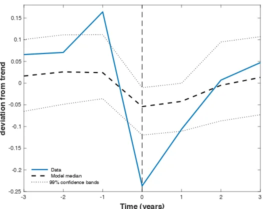
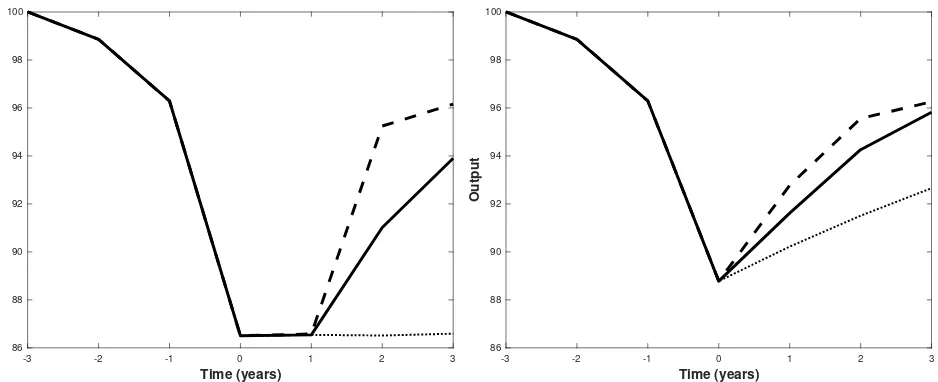
5.2. Output dynamics around defaults
446
One contribution of this paper is to provide a framework able to deliver endogenous output
447
declines in default periods. Figure 2 shows the behavior of output around defaults: the model
448
does feature a decline in output (and consequently in consumption) in the default period. The
449
size of the output drop accounts for 53% of the observed output drop in the data. 23
450
The model also produces a v-shape behavior of output around defaults. Argentina’s output
451
dynamics before and after the default event mostly lie within the 99% confidence bands of the
452
model simulations. As in Mendoza and Yue (2012), the v-shaped recovery of output after a
453
default event is driven by two forces: TFP and re-access to credit. TFP is mean-reverting
454
and thus very likely to recover after defaults. Also, when the sovereign regains access to credit
455
markets, then the output recovery is even faster. 24
456
5.3. Endogenous costs of defaults: credit contractions
457
Why does a default generate such a sharp output decline? This paper gives a credit crunch
458
explanation: given that bankers hold government debt as part of their assets, when a default
459
comes a considerable fraction of those assets losses value; thus, the bankers’ lending ability
460
decreases and as a consequence credit to the private sector contracts. Given that the productive
461
sector is in need of external financing, a credit crunch translates into an output decline.
462
Figure 3 presents the behavior of the Private Credit simulated series around defaults. 25 It
463
shows that credit to the private sector falls in the default period and continues falling in the
464
subsequent periods. The magnitude of the credit drop accounts for 20% of the observed credit
465
drop in the data; in other words, credit plays a more important role in the model economy than
466
in the data.
467
22
This result is by no means new in the literature and it is in fact a consequence of more general capital market imperfections. See Cuadra et al. (2010) and Riascos and V´egh (2003).
23
Figure 2 is constructed from the model simulations as follows: first, we identify the simulation periods when defaults happen; secondly, we construct a time series of 11 years before and 4 years after each default and compute deviations from trend; thirdly, we compute relevant quantiles and construct a series for the median output deviations from trend around defaults; fourthly, we plot deviations from trend generated by the model and those observed in the data for thet−3 tot+ 3 time window, withtdenoting the default year.
24
See the Online Appendix for an analysis of the effects of market re-access on output and credit recovery.
25
5.3.1. Two properties of the output cost of defaults
468
Here we analyze two properties of the output costs of default: that they are increasing in
469
the level of TFP and that they are increasing also in the size of the default (i.e. the level of
470
outstanding debt that is repudiated).
471
Using the numerical solution of the model we are able to compute the effect of defaults on
472
output. The left panel of Figure 4 shows the percent decline of output as a function of TFP.
473
26 As the figure shows, the cost increases with the level of TFP. This property (referred to
474
in the literature as “asymmetric cost of defaults”) is shared by other papers with endogenous
475
cost-of-default structures (e.g. Mendoza and Yue, 2012) and has been shown to be critical to
476
match the counter-cyclicality of sovereign spreads: in good times (high TFP) defaulting is too
477
costly, investors understand this and assign a low probability to observing a default event, this
478
translates into low spreads; on the contrary, during bad times (low TFP) defaulting is less
479
costly (and therefore a more attractive policy choice), defaults are more likely and spreads are
480
consequently higher. 27
481
A second property of the cost of defaults is that they are an increasing function of the level of
482
debt. This has a clear intuition: the more debt a government repudiates, the higher the cost of
483
repudiation. Our framework is to our knowledge the first quantitative model that endogenously
484
delivers this behavior (which is supported by the data, see Arellano et al., 2013). The right
485
panel of Figure 4 shows how the output cost of defaults increases with the level of outstanding
486
debt.28 This happens because sovereign debt plays a “liquidity” role in our economy: the more
487
debt is repaid, the more funds can be lent in the private credit market, and the lower is the
488
equilibrium interest rate paid by firms. As explained above, a credit crunch translates into an
489
output decline, and the larger is the stock of repudiated debt, the larger the credit crunch. 29
490
26
The shaded area in the left panel of Figure 4 represents the “default region,” which are the levels of TFP shock at which the country decides to default when facing the mean debt-to-output level and the mean bank storage observed in the simulations.
27
Chatterjee and Eyigungor (2012) provide a detail discussion about the asymmetric nature of default costs. They use an ad hoc cost-of-default function (in an endowment-economy model) and their calibration implies the same asymmetry that our model delivers endogenously.
28
The shaded area in the right panel of Figure 4 represents the “default region,” which (in this case) are debt-to-output levels for which the country decides to default when facing the mean TFP and the mean bank storage levels.
29
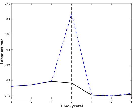
5.4. Benefit of defaults: reduced taxation
491
As argued in the introduction, the optimal default decision comes from balancing costs and
492
benefits of defaults. The costs of default were discussed above: output declines due to a credit
493
contraction. The benefits on the other hand come from reduced taxation. Figure 5 shows the
494
behavior of the labor income tax rate around defaults: we plot the equilibrium tax rate and also
495
the “counterfactual” tax rate that would have been necessary to levy if instead of defaulting
496
the government had repaid its debt.
497
The reduced taxation is precisely the difference between the counterfactual tax rate and the
498
equilibrium tax rate: this difference is of roughly 20 percentage points on average. This tax
499
decline represents a benefit of defaulting because households dislike increases in distortionary
500
taxes. In other words, a default allows the government to afford a tax cut.
501
This subsection and the previous one show that the planner finds a strategic default to be the
502
optimalcrisis resolution mechanism: due to worsening economic conditions, the sovereign finds
503
it optimal to default on its obligations (and assume the associated costs) instead of increasing
504
the tax revenues required for repayment. 30
505
5.5. Sovereign bonds market
506
As discussed above, the model performs quite well with respect to the sovereign bond market
507
dynamics: it produces defaults in bad times and therefore countercyclical spreads. Figure 6
508
shows the equilibrium default region (in the left panel) and the combinations of spreads and
509
indebtedness levels from which the sovereign can choose (in the right panel). With respect to
510
the left panel, the white area represents the repayment area: it is increasing with the level
511
of productivity and decreasing with the level of indebtedness. The right panel presents the
512
spreads schedule that the government faces. As expected, the spreads that the government can
513
choose from increase with the level of indebtedness and decrease with the level of productivity.
514
The model also features a positive correlation between spreads and the debt-to-output ratio,
515
as seen in the data. From Figure 6 we can see that default incentives increase with the debt ratio,
516
hence bond prices are decreasing with the debt ratio (which results in the positive correlation
517
30
between spreads and debt ratios). 31
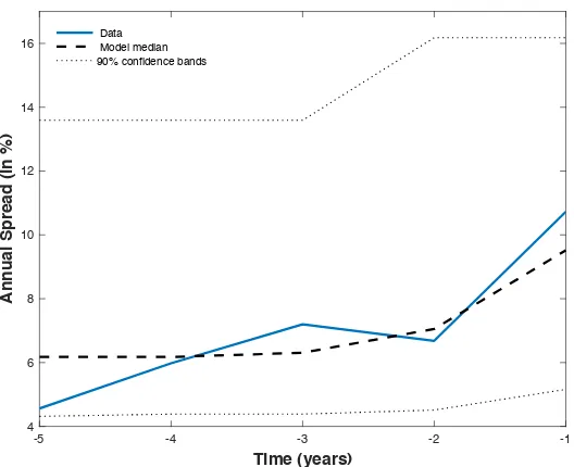
518
Next we turn to the behavior of spreads in the run-up to a default. Figure 7 shows that the
519
spreads generated by the model mimic the behavior of the Argentine spreads, in that they are
520
relatively flat until the year previous to a default, when they spike. The spreads dynamics in
521
the run-up to a default, as seen in the data, are well within the 99% confidence bands of the
522
model simulations.
523
6. Robustness
524
In this section we study the robustness of our results to two modifications. First, we show
525
that the main results are robust to a calibration featuring a lower exposure ratio. Secondly,
526
we study a model with stochastic bankers’ endowment and also show that the main results
527
are robust to this extension. The online appendix contains a thorough parameter sensitivity
528
analysis and also provides a brief discussion about the quantitative relevance of some of our
529
simplifying assumptions.
530
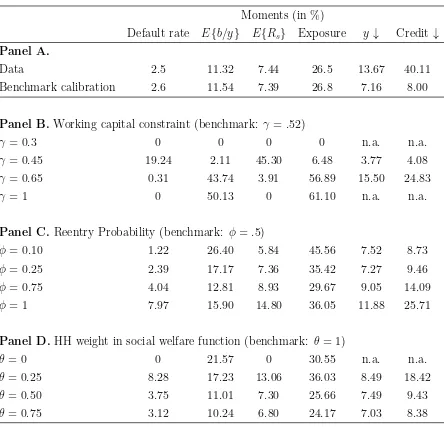
6.1. Calibration to a lower exposure ratio
531
In a recent paper, Gennaioli et al. (2016) report an average exposure ratio of 9.3% when
532
using the entire Bankscope dataset (covering both advanced and developing countries). When
533
they focus only on defaulting countries, they find an exposure ratio that is roughly 15%. In this
534
subsection we re-calibrate our model to feature a lower exposure ratio close to this magnitude
535
and refer to this version as the “low-exposure” economy. 32
536
Table 3 shows selected moments of the data, the benchmark economy and the low-exposure
537
economy. We can see that the dynamics of the sovereign debt market remain mostly unchanged.
538
At a virtually identical default frequency (which was a targeted moment), the low-exposure
539
economy has a mean debt-to-output ratio of 6.39% (which represents 55% of the ratio obtained
540
in the benchmark economy and 56% of the observed ratio). The lenders understand that,
541
31
While it is true that higher debt makes the cost of default higher (see Section 5.3.1), it is also true that higher debt makes the benefit of defaulting higher: the counterfactual tax break that households enjoy during defaults is larger with larger debt stocks. Hence, what matters for the correlation between spreads and debt is the net effect on default incentives.
32
with a higher A (i.e. a higher bankers’ endowment), debt is less important for the functioning
542
of private credit markets and therefore the planner has a higher temptation to default on it,
543
therefore they reduce sovereign lending. They equilibrium spread is almost identical across the
544
two simulated economies, but more volatile for the low-exposure calibration. 33
545
As the theory predicts, an economy with a lower exposure ratio has a lower debt-to-output
546
ratio, should experience a smaller credit crunch and consequently exhibit milder output drops
547
at defaults. Along these lines, we see from Table 3 that the low-exposure calibration can explain
548
only 44% of the output decline at defaults (5.95% versus the observed 13.67%).
549
The main difference between this low-exposure economy and the benchmark economy is
550
quantitative: the lower exposure ratio implies (in line with the theory) that the credit and
551
output drops are smaller. However, the main mechanisms are still present qualitatively and in
552
some dimensions even quantitatively.
553
6.2. Stochastic bankers’ endowment
554
A simplifying assumption used so far was to model banker’s endowment as a constant.
555
However, there is enough evidence showing that bank funding does move with cycle, and this
556
may have interesting implications for our study. In particular, movements inA can change the
557
quantitative effect of defaults and alter the default incentives: for example, a high level of A
558
makes debt repayment less important for the credit supply (i.e. lower output cost of default)
559
and therefore increases the temptation to default.
560
To quantify the effect that movements in A may have we extend the benchmark model and
561
introduce the following functional form for banker’s endowment, following Mallucci (2015):
562
At=a0+a1zt. (26)
In this subsection we re-calibrate our model and refer to this version as the “stochastic–A”
563
economy. 34 The last column in Table 3 has the results for this version of the model. The
564
33
Other non-targeted business cycle moments (not reported in Table 3), like relative volatilities and correla-tions with output, are also in line with the data.
34
We calibrate parameters {a0, a1} to match the mean (26.5%) and the standard deviation (2%) of the
exposure ratio. The calibrated values are a0 = 0.16, and a1 = 0.045. The stochastic–A version approximates
behavior of the sovereign debt market is very similar to the one in the benchmark calibration:
565
spreads are large and volatile, and the mean debt level is also in line with the data. Both the
566
credit and the output drops are somewhat magnified, and so in that dimension the stochastic-A
567
economy is closer to the Argentine evidence explaining 55% of the output decline and 25% of
568
the credit crunch. Overall, the quantitative predictions of the model remain robust to this
569
extension.
570
7. Conclusions
571
The prevalence of defaults and banking crises is a defining feature of emerging economies.
572
Three facts are noteworthy about these episodes: (i) defaults and banking crises tend to happen
573
together, (ii) the banking sector is highly exposed to government debt, and (iii) crisis episodes
574
involve decreased output and credit.
575
In this paper, we have provided a rationale for these phenomena. Bankers who are exposed
576
to government debt suffer from a sovereign default that reduces the value of their assets (i.e.,
577
a banking crisis). This forces the bankers to decrease the credit they supply to the productive
578
private sector. This credit crunch translates into reduced and more costly financing for the
579
productive sector, which generates an endogenous output decline.
580
The benchmark calibration of the model produces a close fit with the Argentine business
581
cycle moments. When calibrated to target the observed default frequency and exposure ratio,
582
the model generates sovereign spreads that compare well with the data, in terms of both levels
583
and volatility. Furthermore, the model features a v-shaped behavior for both credit and output
584
around defaults, which is consistent with the data. The mechanism proposed in the paper is
585
able to account for 53% of the observed GDP drop and 20% of the observed credit drop around
586
default periods.
587
This paper quantifies the impact of a sovereign default on the domestic banks’ balance
588
sheets, their lending ability and economy-wide activity. Its chief methodological contribution is
589
that it presents an endogenous default cost that works through a general-equilibrium effect of
590
the government’s default decision on the economy’s working-capital interest rate. Additionally,
591
ours is the first quantitative paper to endogenize the output cost of default as a function of
592
repudiated debt. This makes our framework a natural starting point for further research on the
593
optimality of fractional defaults.
References
595
Acharya, V., Drechsler, I., Schnabl, P., 2014. A pyrrhic victory? bank bailouts and sovereign
596
credit risk. The Journal of Finance 69, 2689–2739.
597
Adam, K., Grill, M., 2017. Optimal sovereign default. American Economic Journal:
Macroe-598
conomics 9, 128–164.
599
Arellano, C., 2008. Default risk and income fluctuations in emerging economies. American
600
Economic Review 98(3), 690–712.
601
Arellano, C., Mateos-Planas, X., Rios-Rull, J.V., 2013. Partial default. Mimeo, U of Minn .
602
Balloch, C.M., 2016. Default, commitment, and domestic bank holdings of sovereign debt
603
Mimeo, Columbia University.
604
Balteanu, I., Erce, A., Fernandez, L., 2011. Bank crises and sovereign defaults: Exploring the
605
links Working Paper. Banco de Espana.
606
Beck, T., Demirguc-Kunt, A., Levine, R., 2010. Financial institutions and markets across
607
countries and over time: The updated financial development and structure database. The
608
World Bank Economic Review 24, 77–92.
609
Bocola, L., 2016. The pass-through of sovereign risk. Journal of Political Economy 124, 879–926.
610
Bolton, P., Jeanne, O., 2011. Sovereign default risk and bank fragility in financially integrated
611
economies. IMF Economic Review 59(2), 162–194.
612
Borensztein, E., Panizza, U., 2009. The costs of sovereign default. IMF Staff Papers 56.
613
Broner, F., Erce, A., Martin, A., Ventura, J., 2014. Sovereign debt markets in turbulent
614
times: Creditor discrimination and crowding-out effects. Journal of Monetary Economics 61,
615
114–142.
616
Brunnermeier, M., Garicano, L., Lane, P., Pagano, M., Reis, R., Santos, T., Van Nieuwerburgh,
617
S., Vayanos, D., 2011. European safe bonds (esbies) Euro-nomics Group.