Inflation is Always and Everywhere an Interest Rate Phenomenon

(1)

Munich Personal RePEc Archive

Inflation is Always and Everywhere an

Interest-Rate Phenomenon

Belanger, Gilles

Ministere des Finances du Quebec

19 April 2016

(2)

Inflation is Always and Everywhere an Interest-Rate

Phenomenon

Gilles B´elanger

∗

April 19, 2016

Abstract

Following an earlier paper, I investigate an economy where nominal interest rates are rigid, but aggregate prices are not. Though the title exaggerates, interest rates

rigidity does account for an uncanny number of stylized facts about inflation. This paper shows that previously shown results are robust to changes in the specification of interest rate rigidity. Results investigated include: (1) the procyclicality of

infla-tion, (2) inflation control through interest rate manipulainfla-tion,(3) the persistence of inflation since World War II, (4) the Great Moderation under inflation targeting,

(5) real rate volatility under a gold standard, (6) the price puzzle.

Keywords: Interest Rate Rigidity, Inflation, Monetary Policy, Fisher Effect.

JEL: E31, E43, E52.

∗_{Ministère des Finances du Québec; 12, rue Saint-Louis, Québec (Québec) Canada, G1R 5L3;}

(3)

1 Introduction

Interest rates provide a natural model of inflation. Inflation is the dynamics of prices, and interest rates are the prices that bind statics and dynamics to a model making the Fisher Equation is a rare determinant of inflation we can work with. The use of the Fisher Equation forces one to posit either price or nominal-interest-rate rigidities for identification purposes: a solution has to come from some sort of rigidity. New Keynesians rely on rigidity in prices themselves, but this paper takes a look at rigidity in interest rates.

B´elanger (2015) introduces a model of inflation through interest rate rigidity where prices are otherwise flexible at least in the aggregate. The model yields results mentioned

in the Abstract. InB´elanger(2015), rigidity come from Rotemberg pricing, but this paper

introduces other specifications to compare with the original results. Absent a solid theory for rigidity, these comparisons help us to explore the numerical properties of nominal interest rate rigidity, and in doing so, facilitate future research on the theory. This is the primary contribution of this paper.

The models for interest rate rigidity we will explore consist of the original Rotemberg

pricing model, two ad hoc model (one with backward-looking rigidity, one with

forward-looking rigidity), and a model with a sole private bank that minimizes interest rate risk and inflation risk. I believe these rigidity models provide a good range of possibilities such that an eventual richer theory will be close to one or a combination of them.

To conduct the assessment, Section 3 presents the same impulse response functions

(IRFs) and simulations as in B´elanger (2015), but for each rigidity model. The shocks

performed for the IRFs consist of surprise and anticipated, temporary and permanent,

shocks to the natural real interest rate and to the central bank’s inflation target.

Sim-ulation of different regimes use the inflation target as a random variable. To simulate a gold standard regime the inflation target variable has a volatile inflation target and no persistence. A fix inflation target to simulate the actual inflation target regime, and a persistent with small volatility target to simulate to period in between the Gold Standard and the Great Moderation.

The justifications of the model stem from shortcomings of available inflation models.

In quantity theories for example, M V = P Q, both M and V are adjustable by agents.

History showed people compensated for lack of species with alternatives, be it cigarettes

in prison or playing cards in New France. So if P is anchored otherwise, M V will adjust

(4)

price level in a static setting as there are no anchors for a num´eraire. Setting prices using the interaction between something that is not an anchor and rigidity on itself is not convincing for me.

The rigidity models, detailed in Section 2, are evaluated by their ability to match

results that Subsection 1.1 presents. Section 3 presents the results.

1.1 Results to be tested

Imagine that financial participants do not fully adjust nominal rates to changes in real rates, or that the central bank has to contend with a financial system plagued with an

in-complete pass-through from real to nominal rates. As shown byEckstein and Sinai(1986),

an important link exists between credit conditions and economic fluctuation. This relation

was recently illustrated byAikman, Haldane and Nelson(2014) and shown empirically by

L´opez-Salido, Stein and Zakraj˘sek (2016). A representative interest rate would include

measures of credit tightness (almost no one borrows at Treasury rates), making r

coun-tercyclical, or rising during recessions. Subsection 3.2.1 shows that the inverse relation

also applies to changes in r that come from the real economy. Since i never quite catch

up to r, recessions will necessarily lead to downward pressures on prices, not because of

demand, but because of the way nominal interest rates are set.

But it also affect the central bank. The central bank’s open market operations, or threats of open market operations, affect real rates more than on nominal rates. Remem-ber, the central bank does not set nominal interest rates, but it achieves the nominal interest rates it wants through its operations. Which brings us to the Fisher Equation,

i =r+π. If i moves in the same direction, but by less than r, then π comes down. As

discussed in Subsection 3.2.2, the central bank facing interest rate rigidity needs to raise

rates to lower inflation or lower them to raise it.

Furthermore, gold prices are so volatile that inflation continually swings back and forth, which the model replicates well. Data from the period shows no persistence in prices. Only when central banks started to worry about inflation did persistence in price appeared as Benati (2008) shows. Since persistence of aggregate prices in New Keynesian models come from the market, why did the market only behave that way after Roosevelt dropped the gold peg? Persistence must have come from the central banks instead. Subsection

3.2.3 discusses persistence.

(5)

inflation-target volatility is high. That means the Gold Standard was not only detrimen-tal to price stability, but to real interest rate stability as well, thus to the real economy. Consequently, a constant inflation target lowers real-interest-rate volatility. As shown in

Subsection3.2.4, this explains the Great Moderation as macroeconomic variable’s

volatil-ity significantly dropped since the mid-eighties when central banks finally resolved to keep

inflation down. SeeStock and Watson (2003) for a discussion of the Great Moderation.

Interest rate rigidity implies other things. B´elanger (2015) shows nominal interest

rates move in the same direction of inflation when the central bank changes its inflation target. The intuition has to do with the Fisher Effect: agents demand higher interest rates to pay for a foreseeable rise in inflation. Imagine an inflation target that keeps changing. This is what happens under a gold standard, essentially an inflation target that changes every day with the price of gold. Under volatile target, inflation would move in the same direction as nominal interest rates when the target changes, but in the opposite direction

with economic fluctuations, as shown in Subsection 3.2.5.

Now, Sims (1992) discovered the price puzzle. It states that an increase (decrease)

in interest rates leads to a rise (fall) of inflation initially; only a later does inflation falls (rises) as expected. Forward-looking models bring dynamics into interest rate setting, so nominal interest rates will react immediately to information about the future. As shown

in Subsection 3.2.6, nominal interest rates will rise now if agents expect a rise in real

interest rates in the future. Equation i = r +π says with i increasing and r not yet

moving, π will temporarily rise untilr itself starts to move, hence the price puzzle.

Finally, Subsection 3.2.7 discusses what happens if there is no monetary policy. One

result from the adjustment costs model is that, because of adjustment costs, no monetary policy means market participants minimize adjustment costs by keeping nominal interest rates constant. That explains why interest rates could stay the same for decades in Ancient times, established by tradition or law.

Of course, there is also the question of the zero lower bound on nominal interest rates. At the zero lower bound, nominal interest rates cannot move and the central bank becomes powerless. The liquidity trap is equivalent to having no monetary policy. Only with luck

or financial repression can we get out of a liquidity trap by sending r to a low enough

(6)

2 The four models and absence of policy

The model uses the “Interest Rate Rigidity” model of inflation. B´elanger (2015) shows

that in a world where recessions are associated with tight credit, interest rate rigidity is sufficient to explain the major stylized facts about inflation.

The framework borrows from Woodford (2003) where the natural interest rate, r∗

t,

comes from r∗

t = k

′

st where s represents the state variables from the real economy and

k, the parameters associated with them. The financial markets consists of two additional

agents, a central bank and a private bank. The private bank set nominal interest rates while the central bank influence real interest rates, and nominal ones indirectly, pursuant to its inflation target.

First, the model uses the Fisher equation or ex-ante definition of real interest rates (in log form),

rt=it−1−πt. (1)

The use of the equation supposes that the model pins down inflation by pinning down real interest rates. Pinning down real interest rates can be done by using an homogeneous production function like a Cobb-Douglas.

Second, a central bank uses a Taylor Rule, but for real interest rates,

rt=r∗

t +µ(πt−π

∗

t). (2)

for a positiveµ, whereπ∗

represents the inflation target.

Note that the setup supposes that the full model uses a homogeneous production function. A homogeneous production function defines ex-post real interest rates by making them what is left after firms pay wages and depreciation. Because of Euler’s theorem, this residue coincides with the marginal product of capital.

The third equation varies across specifications. The following subsections present them.

2.1 Model I and II: Ad hoc models

In Model I, we use a simple lag specification, where nominal interest rates move in anad

hoc manner without theoretical justification.

it=δit−1+ (1−δ)Et[r

∗

t+1+π

∗

(7)

where nominal interest rates gradually move toward its natural state that consists of the natural real interest rate plus the inflation target.

In model II, we use a simple lead specification, again without theoretical justification.

it=δE[it+1] + (1−δ)Et[r

∗

t+1+π

∗

t+1] (4)

A fuller justification would anyway need a few shortcuts. It is best to simply pose the form, as this form is a natural benchmark with which to compare the other models presented here.

2.2 Model III: Adjustment costs

In the adjustment costs specification, taken fromB´elanger(2015), a private bank set

nom-inal interest rates under adjustment quadratic costs to nomnom-inal interest rates (Rotemberg pricing, but in nominal interest rates) and a quadratic costs of real rates distortion,

min it ( Et "∞ X s=0 βs

rt+1+s−r

∗

t+1+s

2

+θ(it+s−it−1+s)

2 #)

.

where θ defines the weight associated to each cost. Using Equations (1) and (2), we can

rewrite the objective function as

min it    Et   ∞ X s=0 βs   µ

1 +µ

!2

rt+1+s−it+s−π

∗

t+1+s

2

+θ(it+s−it−1+s)

2        .

Optimization by the private bank leads to the following evolution equation for nominal interest rates,

∆it =βEt∆it+1+

1

θ µ

1 +µ

!2

Et

h

r∗

t+1+π

∗ t+1 i −it . (5)

One can readily see that in the absence of monetary policy, if µ = 0, nominal interest

rates will not move. See Section 2 ofB´elanger(2015) for the justification and a discussion

of the model.

2.3 Model IV: The Pareto Bank

(8)

The bank sets nominal interest rates at a Pareto optimum given the prevailing real rate. The bank does not set real rates this way because they come as given from the real economy. Borrowers and lenders are price takers when confronted by intertemporal preferences and the marginal productivity of capital.

Changes in real interest rates either translate to changes in nominal interest rates, inflation, or both. Pass-through from real to nominal rates is incomplete when inflation is used. Since reinvestment neutralizes the effects of changes in nominal interest rates, people who intend to hold a debt or bond until maturity only fear unexpected inflation, or inflation risk. Others fear both interest rate risk and inflation risk. Therefore, in the short term, we witness a compensation mechanism. If interest rate risk and inflation risk were the only things in play, the equation would take the form of

Et−j[it]−Et−j−1[it] =

∞

X

s=j βs_λt,t

+s

1− ηt,t+s 2

(Et−j[rt+1+s]−Et−j−1[rt+1+s]), (6)

where β represents the discount factor, λt,t+s, the fraction of debts at time t that have

maturities at or beyond t+s, andηt,t+s, the expected fraction of debts or bonds in λt,t+s

expected to be sold or reimbursed at time t+s.

To simplify, we pose that βs_λt,t

+s(1−ηt,t+s/2) = ζγs, so

Et−j[it]−Et−j−1[it] =

∞

X

s=0

ζγs_(E

t−j[rt+1+s]−Et−j−1[rt+1+s]).

This can be solved recursively by noting that Et−j[xt] is the steady state whenj tends to

infinity, yielding

it−¯ı=

∞

X

s=0

ζγs_E

t[rt+1+s]−ζ(1−γ)

−1 ¯

r.

For coding purposes, pose a Bellman equation. Define V such that

Vt=

∞

X

s=0

ζγs_E

t[rt+1+s] =ζEt[rt+1] +γEt[Vt+1],

and replace steady states with the expectation many period in advance (instead of ¯x, use

Et[xt+k] for large k, I use k= 100).

2.4 No monetary policy

The case of no monetary policy is not so much a rigidity model as a good point of comparison. Model III offers a clear argument in case there is no monetary policy. To

compare with this case, we simply imposeµ= 0, so the model is reduced to

(9)

Table 1: Parameter values

symbol value

Steady state inflation target π¯∗

0.0075

Steady state real interest rate ¯r∗

0.005

Monetary policy tightness µ 0.5

Rate persistence – Model I & II δ 0.75

Discount factor – Model III β 0.995

Adjustment cost – Model III θ 1

Drop parameter – Model IV γ 0.9

Level parameter – Model IV ζ 0.1

Furthermore, we suppose that an outside force like the government or tradition imposes

it= ¯ıwhich means that for rt= ¯r, we have πt = ¯π and ¯ı= ¯r+ ¯π.

3 Comparing results

The Section shows what results from the interest rate rigidity survive changes in

specifi-cation. The results in question each have their own Subsection: 3.2.1) the procyclicality

of inflation, 3.2.2) inflation control through interest rate manipulation, 3.2.3) inflation

persistence in modern times,3.2.4) the Great Moderation,3.2.5) real rate volatility under

a gold standard, 3.2.6) the price puzzle and3.2.7) the case of no monetary policy.

3.1 The setup

The setup mirrors that of B´elanger (2015) where r∗

, from equation (2), consists of the

sum of two exogenous shocks,

r∗

t = ¯r

∗

+εa

t−4+ε

s

t, (7)

where εa _{represents an anticipated shock (four periods in advance),} _εs_{, a surprise shock}

and ¯r∗

, the steady state real interest rate. Both shocks follow first-order autoregressive processes.

IRFs and simulations share the same non-shock parameters, listed in Table 1. The

justifications of the parameter values are straightforward. The adjustment cost parameter,

θ, is set at the non-committal value of 1. The discount factor,β, is set at 0.995 so ¯r∗

equals

β−1

(10)

Table 2: Shock parameter values

standard deviation persistence

Surprise real interest rate shock 0.005 0.6

Anticipated real interest rate shock 0.005 0.6

Inflation target shocks

... under gold standard regime 0.13 -0.05

... under non-target fiat regime 0.004 0.975

... under inflation target regime 10−8

0

quarter to make the results readable in the figures. For IRFs, the persistence parameters

for the shocks are ρ= 0.75 for temporary shocks and ρ= 0.999999 for permanent shocks

(not exactly 1 to secure a numerical solution).

The monetary regimes are thus: a gold standard with a volatile inflation target, which replicates the regime’s high volatility in ex-post real interest rates; a non-target fiat regime with a very persistent inflation target process, replicating the non-stationarity seen in nominal interest rates and the more persistent ex-post real rates; and an inflation target regime with a constant inflation target.

For all simulations, surprise and anticipated real-interest-rate shocks respectively

fol-low processes each with 0.6 persistence and standard deviations of 0.005. Table2lists the

shock-parameter values applied to the regimes; I discuss them in turn with each regime.

3.2 The results

The results appear on the Figures at the end of the paper. Responses under different models coincide quantitatively whether they pertain to the temporary shocks responses

of Figures1, 2 and 3 and the permanent shocks of Figures 4,5 and 6. Most support the

(11)

steady state almost instantly. Fifth and finally, Model IV, with the Pareto bank, sees nominal interest rates move in the same direction of real interest rates for a temporary shock to the inflation target. Although, this is not a recognized stylized fact, all other models see real and nominal interest rates move in opposite direction in reaction to an inflation-target shock. Still, the opposite movements of interest rates — unique to between 1950 and 1990 — militate for the movements coming from changes in the inflation target. Thus, they are a nice feature of the interest rate rigidity model.

Figures 7, 8 and 9 present the output to simulated monetary regimes. They all

re-produce the main features of the regimes they are simulating though the amplitudes of interest rate movement vary a little.

For its part, Table 3 presents the main statistics of the simulated variables for the

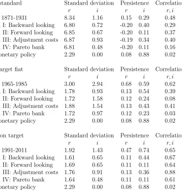
different models and regimes. The statistics stems from autoregressive model applied to the simulation results to yield measures for standard deviations, persistence and correla-tions. Results vary little from model to model. The only significant difference come in the correlation numbers where Model IV displays no correlation between rates under a gold standard, and both Model II and IV display slightly negative correlation between real and nominal interest rates unlike other model where the correlation is positive.

3.2.1 The procyclicality of inflation

In the model, an increase in real interest rates leads to a drop in inflation. Research is confirming that credit conditions are anticyclical meaning real interest rates paid by firms and people increases, unlike headline interest rates characterized by private banks’ prime rates or by central banks’ key rate. Hence, the procyclicality of inflation.

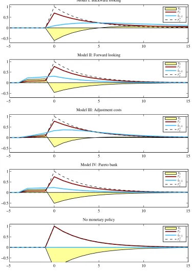
Figure1shows the response of the nominal interest rate and inflation to an exogenous

change in real interest rate. Note that the real interest rate partly reflects the initial one-percent shock, and partly the feedback from monetary policy. The figure shows the muted response of the nominal interest rate and the subsequent drop in inflation.

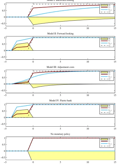
Figure 4shows the same response, but to a permanent shock. In this case, Models II

and IV clearly fail. Deflation only lasts one quarter as agent adjust immediately. Other models fare well.

In the cases of the anticipated shocks, in Figures 2 and 5, the failures and successes

(12)

3.2.2 Inflation control through interest rate manipulation

A central bank uses market operations, or the threat of them, to influence nominal inter-est rates. But the operations will influence nominal rates only indirectly through their influence on real rates, the rates that economic agents care about. When nominal rates only partially react to real rates and prices are flexible, as posited here, inflation moves in the opposite direction to interest rates. Therefore, the central bank needs to increase interest rates to lower inflation.

Because of internalized monetary policy, we must show the impact of a central bank by comparing a version of the model with or without monetary policy. In the absence of monetary policy, nominal interest rates will not move, so a change in real interest rates, shown in the dotted lines, translates perfectly to the opposite change in inflation. We see

success in the distance between the rt and r∗

in the Figures 1, 4,2 and 5.

The figures show the same models succeed or fail at the same places as in the previ-ous section. Of course, both the procyclicality of inflation and inflation control through interest rate manipulation are essentially the same problem.

3.2.3 Inflation persistence in modern times

Inflation persistence is new as there is little evidence of it in the pre-War era. The model shows that under a gold standard, prices will display the persistence of the price of gold, the de facto inflation target. Only in the 1930s did central banks start caring about inflation, only in the 1930s does inflation persistence show up. This is a strong point of the theory: if price persistence comes from the market, as posited by New Keynesians, why the sudden appearance of it?

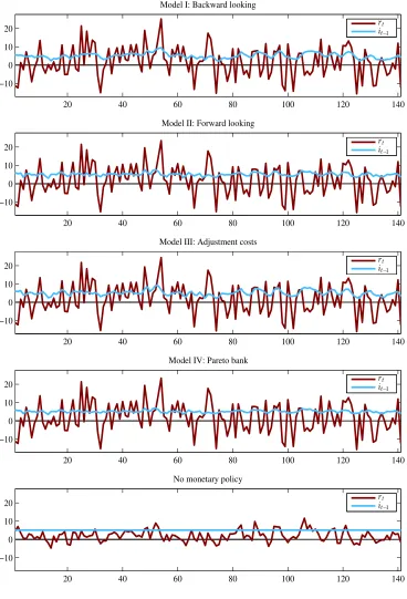
To see this, we must refer to the simulations in Figures 7, 8 and 9, showing how the

gold standard regime is detrimental to price stability. Inflation in all specifications varies

wildly under a gold standard compared to the other two regimes. As Table 3 shows,

the persistence of inflation is a fiat currency phenomenon in the data which all model reproduce.

3.2.4 The Great Moderation

(13)

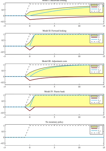
Figure3shows the disrupting effects of a change in the inflation target. The disruption does not prove per say that a change in the inflation target goes against stability, but

it will necessarily go against stability if the changes are random.1

Figure 9 illustrates

how smaller the variance of real interest rates are under a fixed inflation target when

compared to the random changes in the target seen in Figures7and8. As Table3shows,

the standard deviation of real interest rates is even lower than the simulated natural interest rate by more than half a percentage point.

3.2.5 Real rate volatility under a gold standard

Gold prices are volatile, and so will the inflation target under a gold standard. The incomplete pass-through from real interest rates to nominal rates leads ex-post real rates to be volatile when the inflation target is volatile.

As with inflation, real interest rates vary a lot under a gold standard. Figures 7, 8

and9 illustrate the variability of real interest rates under a gold standard compared with

the other regimes. As Table3shows, the standard deviation of the real interest rate over

around 8 percent per year for all models, that is 5 percentage points higher than the natural interest rate taken from the no monetary policy case.

3.2.6 The price puzzle

The price puzzle states that an increase in interest rates initially leads to an increase in inflation a few quarters before inflation finally drops as expected. Under the model, the price puzzle implies that agents modify nominal interest rates immediately when they expect any future changes in real interest rates. With the immediate change in nominal rate not associated with a change in real rates, inflation will rise because of the Fisher equation, and this rise will last until real rates finally changes.

Figures 2 and 5 show that Model I fails to generate the initial inflation. This is due

to the necessity to have forward-looking behavior solve the price puzzle.

3.2.7 No monetary policy or the zero lower bound

For real interest rate shocks, the dotted lines in Figures1,4,2and5represent no monetary

policy or interest rates at the zero lower bound. The dotted lines show that rt=r∗

t at all

1_{That is unless they aim at lowering real rate volatility. Such policy is well beyond the scope of the}

(14)

time since the absence of monetary policy which corresponds to µ = 0 in the monetary

policy equation, equation (2).

Note that for Model III, the case is clear and detailed in B´elanger (2015) for both

the Rotemberg pricing interpretation of the model and the Calvo pricing one. For that

reason, Model III, with µ= 0, is used for the no monetary policy case.

4 Conclusion

The paper shows that nominal interest rate rigidity yields interesting results independent of how we model said rigidity. For three models of rigidity in nominal interest rates, most result holds up. The three models consists of (I) a simple lag specification, (II) a simple lead specification, (III) quadratic adjustment costs `a la Rotemberg, and (IV) a Pareto bank. The results consists of (1) the procyclicality of inflation, (2) inflation control through interest rate manipulation, (3) the persistence of inflation since World War II, (4) the Great Moderation under inflation targeting, (5) real rate volatility under a gold standard, (6) the price puzzle.

Each model satisfies many of the results. The results that do not pan out lead to the conclusion that the rigidity equation needs a forward looking form to account for the price puzzle, and that the forward looking form cannot be neutralizing to the point where all information about the future get internalized immediately.

As these results show, the form or justification of rigidity is not critical to the central point that nominal interest rate rigidity in itself explain most stylized facts about inflation. The overwhelming mass of results should make us reconsider the underlying causes of inflation movements.

Furthermore, the paper provides a good complement, and maybe an introduction, to

the interest rate rigidity theory of inflation presented in B´elanger (2015). It also serves

as an early, albeit fragmentary, exploration of interest rate rigidity.

References

Aikman, David, Andrew G. Haldane and Benjamin D. Nelson (2014),“Curbing the Credit

(15)

B´elanger, Gilles (2015), “Interest Rate Rigidity and the Fisher Equation,” Available at SSRN, No. 2444280.

Benati, Luca (2008),“Investigating Inflation Persistence Across Monetary Regimes,” The

Quarterly Journal of Economics, 123(3), pp. 1005–1060.

Eckstein, Otto and Allen Sinai (1986), “The Mechanisms of the Business Cycle in the

Postwar Era,” inThe American Business Cycle: Continuity and Change, ed. Robert J. Gordon, chapter 1, pp. 39–122, Cambridge: National Bureau of Economic Research.

L´opez-Salido, David, Jeremy C. Stein and Egon Zakraj˘sek (2016), “Credit-Market

Sen-timent and the Business Cycle,” NBER Working Papers 21879, National Bureau of Economic Research, Inc.

Sims, Christopher A. (1992), “Interpreting the macroeconomic time series facts: The

effects of monetary policy,” European Economic Review, 36(5), pp. 975–1000.

Stock, James H. and Mark W. Watson (2003), “Has the Business Cycle Changed and

Why?” inNBER Macroeconomics Annual 2002, eds. Mark Gertler and Kenneth Rogoff, volume 17, pp. 159–230, MIT Press.

Woodford, Michael (2003), “Optimal Interest-Rate Smoothing,” Review of Economic

(16)

[image:16.612.116.474.169.546.2]

A

Tables and figures

Table 3: Standard deviations and correlation

Gold standard Standard deviation Persistence Correlation

r i r i r, i

Data: 1871-1931 8.34 1.16 0.15 0.29 0.48

Model I: Backward looking 6.80 0.72 -0.20 0.40 0.29

Model II: Forward looking 6.85 0.67 -0.20 0.11 0.37

Model III: Adjustment costs 6.87 0.93 -0.19 0.34 0.40

Model IV: Pareto bank 6.81 0.48 -0.20 0.11 0.16

No monetary policy 2.29 0.00 0.08 0.88 0.02

Non-target fiat Standard deviation Persistence Correlation

r i r i r, i

Data: 1965-1985 3.00 2.94 0.68 0.59 0.62

Model I: Backward looking 1.78 0.93 0.13 0.54 0.39

Model II: Forward looking 1.72 1.58 0.12 0.24 0.08

Model III: Adjustment costs 1.88 1.54 0.13 0.43 0.41

Model IV: Pareto bank 1.72 0.97 0.12 0.23 0.03

Inflation target Standard deviation Persistence Correlation

r i r i r, i

Data: 1991-2011 1.92 1.43 0.47 0.74 0.65

Model I: Backward looking 1.61 0.65 0.11 0.44 0.67

Model II: Forward looking 1.69 0.65 0.11 0.11 0.64

Model III: Adjustment costs 1.76 0.91 0.13 0.36 0.88

Model IV: Pareto bank 1.64 0.48 0.11 0.11 0.61

(17)

[image:17.612.120.495.128.659.2]

Figure 1: Temporary one percent surprise real interest rate shock responses

−5 0 5 10 15

−0.5 0 0.5 1

Model I: Backward looking

π_t

rt

it₋₁

r∗ t

−5 0 5 10 15

−0.5 0 0.5 1

Model II: Forward looking

πt

rt

i_t

−1

r∗ t

−5 0 5 10 15

−0.5 0 0.5 1

Model III: Adjustment costs

πt

rt

it₋₁

r∗ t

−5 0 5 10 15

−0.5 0 0.5 1

Model IV: Pareto bank

π_t

rt

it₋₁

r∗ t

−5 0 5 10 15

−0.5 0 0.5 1

No monetary policy

πt

r_t i_t

−1

r∗ t

Note_{: the vertical axis represents the inflation rate (}π_t_{), the ex post real interest rate (}r_t_{), the nominal}

interest rate (i_t

−1) and the original shock (r∗) in percent deviation from control state; the horizontal axis

(18)

[image:18.612.120.495.128.659.2]

Figure 2: Temporary one percent anticipated real interest rate shock responses

−5 0 5 10 15

−0.5 0 0.5 1

π_t

rt

it₋₁

r∗ t

−5 0 5 10 15

−0.5 0 0.5 1

πt

rt

i_t

−1

r∗ t

−5 0 5 10 15

−0.5 0 0.5 1

πt

rt

it₋₁

r∗ t

−5 0 5 10 15

−0.5 0 0.5 1

π_t

rt

it₋₁

r∗ t

−5 0 5 10 15

−0.5 0 0.5 1

No monetary policy

πt

r_t i_t

−1

r∗ t

interest rate (i_t

(19)

[image:19.612.120.495.128.659.2]

Figure 3: Temporary one percent surprise inflation target shock responses

−5 0 5 10 15

−0.5 0 0.5 1

π_t

rt

it₋₁

π∗

t

−5 0 5 10 15

−0.5 0 0.5 1

πt

rt

i_t

−1

π∗

t

−5 0 5 10 15

−0.5 0 0.5 1

πt

rt

it₋₁

π_t∗

−5 0 5 10 15

−0.5 0 0.5 1

π_t

rt

it₋₁

π∗

t

−5 0 5 10 15

−0.5 0 0.5 1

No monetary policy

πt

r_t i_t

−1

π∗

t

interest rate (i_t

−1) and the original shock (π∗) in percent deviation from control state; the horizontal axis

(20)

[image:20.612.121.494.127.660.2]

Figure 4: Persistent one percent surprise real interest rate shock responses

−5 0 5 10 15

−0.5 0 0.5 1

π_t

rt

it₋₁

r∗ t

−5 0 5 10 15

−0.5 0 0.5 1

πt

rt

i_t

−1

r∗ t

−5 0 5 10 15

−0.5 0 0.5 1

πt

rt

it₋₁

r∗ t

−5 0 5 10 15

−0.5 0 0.5 1

π_t

rt

it₋₁

r∗ t

−5 0 5 10 15

−0.5 0 0.5 1

No monetary policy

πt

r_t i_t

−1

r∗ t

interest rate (i_t

(21)

[image:21.612.120.494.128.659.2]

Figure 5: Persistent one percent anticipated real interest rate shock responses

−5 0 5 10 15

−0.5 0 0.5 1

π_t

rt

it₋₁

r∗ t

−5 0 5 10 15

−0.5 0 0.5 1

πt

rt

i_t

−1

r∗ t

−5 0 5 10 15

−0.5 0 0.5 1

πt

rt

it₋₁

r∗ t

−5 0 5 10 15

−0.5 0 0.5 1

π_t

rt

it₋₁

r∗ t

−5 0 5 10 15

−0.5 0 0.5 1

No monetary policy

πt

r_t i_t

−1

r∗ t

interest rate (i_t

(22)

[image:22.612.121.495.127.659.2]

Figure 6: Persistent one percent surprise inflation target shock responses

−5 0 5 10 15

−0.5 0 0.5 1

π_t

rt

it₋₁

π∗

t

−5 0 5 10 15

−0.5 0 0.5 1

πt

rt

i_t

−1

π∗

t

−5 0 5 10 15

−0.5 0 0.5 1

πt

rt

it₋₁

π_t∗

−5 0 5 10 15

−0.5 0 0.5 1

π_t

rt

it₋₁

π∗

t

−5 0 5 10 15

−0.5 0 0.5 1

No monetary policy

πt

r_t i_t

−1

π∗

t

interest rate (i_t

−1) and the original shock (π∗) in percent deviation from control state; the horizontal axis

(23)

[image:23.612.125.493.125.666.2]

Figure 7: Gold standard simulation

20 40 60 80 100 120 140

−10 0 10 20

rt

it₋₁

20 40 60 80 100 120 140

−10 0 10 20

rt

it₋₁

20 40 60 80 100 120 140

−10 0 10 20

r_t i_t

−1

20 40 60 80 100 120 140

−10 0 10 20

rt

it₋₁

20 40 60 80 100 120 140

−10 0 10 20

No monetary policy

rt

it₋₁

Note_{: the vertical axis represents the inflation rate (}πt), the ex post real interest rate (rt) and the nominal

interest rate (it₋₁) in percent deviation from control state; the horizontal axis indicates quarters to or

(24)

[image:24.612.127.496.129.655.2]

Figure 8: Non-target fiat simulation

20 40 60 80 100 120 140

−10 0 10 20

rt

it₋₁

20 40 60 80 100 120 140

−10 0 10 20

rt

it₋₁

20 40 60 80 100 120 140

−10 0 10 20

r_t i_t

−1

20 40 60 80 100 120 140

−10 0 10 20

rt

it₋₁

20 40 60 80 100 120 140

−10 0 10 20

No monetary policy

rt

it₋₁

(25)

[image:25.612.126.494.128.654.2]

Figure 9: Inflation target simulation

20 40 60 80 100 120 140

−5 0 5 10

rt

it₋₁

20 40 60 80 100 120 140

−5 0 5 10

rt

it₋₁

20 40 60 80 100 120 140

−5 0 5 10

r_t i_t

−1

20 40 60 80 100 120 140

−5 0 5 10

rt

it₋₁

20 40 60 80 100 120 140

−5 0 5 10

No monetary policy

rt

it₋₁