Abstract—The present work describes the design and analysis of an artificial control of standing and leg articulation system in an efficient way. The total system under consideration is supposed to consist of the muscle dynamics in cascade with suitable compensator operated in the closed loop manner with unity negative feedback path, affording the suitable spatial output of the muscle to the input as available from the body input. The optimality of the performance for the system is considered to be attained with gain of the (PID) compensator so chosen that the integral square error becomes a minimum. The overall system is found to be stable, controllable and observable. The system is also analyzed in sampled data control domain (z domain). The stability in z domain is analyzed using Jury’s Stability test. MATLAB software is appropriately used in the entire analysis. The overall system offers an indepth sight for the biomedical engineering application of an artificial control of standing and leg articulation system operated in optimal condition.
Index Terms—Stability, PID compensator, Integral Square Error, Sample data control.
I. INTRODUCTION
The study of the overall system with the use of control theory demands insight into neurophysiology. Muscle control phenomenon is essentially caused by the feedback action of muscle spindle and by sensors based on a combination of muscle length and rate of change of muscle length.
R(s) Y(s)
⊗
±
Fig.1: Block Diagram of artificial control of Standing and leg articulation.
G1(s) =k (s2+s+1) / s; G2(s) =1/s; G3 (s) = 15/ (s2+8s+144);
H (s) =1;
R(s) =leg angle, Y(s) =Desired leg angle.
The analysis of muscle regulation has been based on the theory of single input, single output (SISO) control system. An example is a proposal that the stretch reflex is an experimental observation of a motor control strategy, e.g.
control of individual muscle length by the spindles. However, the regulation of individual muscle stiffness (as available by sensors of both length and force) occurs as the motor control strategy [1].
One model of the human standing balance mechanism is shown in the Fig.1 [2].Case of a paraplegic is considered having lost his control of standing mechanism. An artificial controller is used to enable the person to stand and articulate his legs
It is known that the muscle contraction depends on energy supplied by ATP. Most of the energy is required to actuate the ratchet mechanism by which the cross bridges pull the actin filament, but small amounts are required for i) pumping calcium from the sacroplasm into the sacroplasmic reticulam, ii)pumping sodium and potassium ions through the muscle fiber membrane to maintain an appropriate ionic environment for the propagation of action potentials[3,4,5].
However, the amount of ATP that is present in the muscle fiber is sufficient to maintain full contraction for less than one second. Fortunately, after the ATP is broken into ADP, The ATP is resphosphorylated to form new ATP within a fraction of second. There are several sources of energy required for this resphosphorylation.
The first source of energy, that is used to reconstitute the ATP is the substance creatine phosphate, which carries a high energy phosphate bond of the creatine phosphate is cleaved, and release energy causing bond of a new phosphate into ADP to reconstitute the ATP. However, the total amount of creatine phosphate is also very little, only five times as greater as ATP. So the combined energy of both the stored ATP and the creating phosphate in the muscle is still capable of causing maximum muscle contraction for no longer than few seconds.
Maximum efficiency of muscle can be realized only when the muscle contracts at the moderate velocity. Muscle atrophy is the reverse of muscle hypertrophy; it results any time a muscle is used only for very weak contractions. When a muscle is enervated, it immediately begins to contract, and the muscle continues to decrease in size subsequently. If the muscle becomes reinnervated during the first three to four months, full functions of the muscle originally returns, but afterwards of denervation some of the muscle fibers usually will be degenerated. Re-innervation after two years rarely results in return of any function at all. Pathological studies show that the muscle fibers have, by that time, been replaced fat and fibrous tissue.
Strong electrical stimulation of denervated muscles, particularly when the resulting contractions occur against load, will delay and in some instances prevent muscle atrophy despite denervation.The procedure is used to keep muscles alive until reinnervation can take place.
Design and Analysis of an Artificial Control of
Standing and Leg Articulation System
Achintya Das, and Mrinmoy Chakraborty
G1(s) G3(s)
H(s)
When a muscle is denervated, its fibers tend to shorten, if the muscle is kept in a shortened position, and even the associated nerves and fasciae shorten. All this is a natural characteristic of protein fibers called “creep”. That is, unless continual movement keeps stretching the muscle and other structures, they will creep toward a shortened length. This is one of the problems in treatment of patients with denervated muscles, such as occur in poliomyelitis or nerve trauma. Unless passive stretching is applied to the muscles, they may become so shortened that even when re-innervated, they will be of little value. But, more important, the shortening can often result in extremely contracted positions of different parts of the body.
II. CONVERSION FROM S-DOMAIN
TO Z-DONAIN [6]
Z-transform helps in the analysis and design of sample data control system, as Laplace transform does in the analysis and design of continuous data control system.
The z-transform
F z
( )
of a sample data control signal(
)
f KT
is defined by the relation:0
( )
(
)
KK
F z
f KT z
∞
−
=
=
∑
. … (1)The above relation is derived from the Laplace transformation as applied to sample data control signal. Assuming
e
sT=
z
be the concerned transformation variable in Laplace Transformation,we have
sT
=
l
nz
i.e.
s
1T
nz
−
=
l
… (2) Using power series expansion ofl
nz
, the above equation becomes:1
1
4
4
344
5...
2
3
45
945
T
s
u
u
u
u
−
=
⎡
−
−
−
⎤
⎢
⎥
⎣
⎦
... (3)Where 1 1
1
1
z
u
z
− −−
=
+
… (4)In general, for any positive integral value of
n
31
1
4
44
2
3
45
945
n n
n
T
ss
u
u
u
u
⎛ ⎞ ⎡
⎤
=
⎜ ⎟ ⎢
−
−
−
⎥
⎝ ⎠ ⎣
⎦
… (5)By using binomial expansion in the above equation for various values of
n
, we may have the transformation froms
to
z
domain.III. INTEGRAL SQUARE ERROR (J) [7]
Instead of the time domain calculation of
J
(integral square error), the complex frequency domain can be used. According to a theorem in mathematics by Parseval2 0
1
( )
( ) (
)
2
j SE jJ
I
e t dt
E s E
s ds
j
π
∞ ∞
− ∞
=
=
∫
=
∫
−
… (6)Where
E s
( )
can be expressed as follows:1
1 1 0
1
1 1 0
...
( )
...
n n n n n nN
s
N s
N
E S
D s
D s
D s
D
− − − −
+ +
+
=
+
+ +
+
… (7)assuming type 1 behavior.
J
follows from complex variable theory. To clarify the effect of system order, the subscript forJ
will be the system order. For an nth –order system.1
( 1)
2
n n n n nB
J
D H
−= −
… (8)Where
H
n andB
n are determinants.H
n is the determinant of then n
×
Hurwitz matrix. The first two rows of the Hurwitz matrix are formed from the coefficients of D(s), while the remaining rows consist of right-shifted versions of the first two rows until then n
×
matrix is formed. Thus we writen-2 1 3 2 1 3 D .
...
...
0
..
0
...
...
n n
n n
n n n
n
D
D
D
D
H
D
D
D
− − − − −⎡
⎤
⎢
⎥
⎢
⎥
⎢
⎥
=
⎢
⎥
⎢
⎥
⎢
⎥
⎣
⎦
… (9)The determinant
B
n is found by first calculating2 2 2
2 2 2 0
( ) (
)
n n...
N s N
− =
s
b
−s
−+ +
b s
+
b
… (10) Then first row of the Hurwitz matrix is replaced by the coefficients ofN s N
( ) (
−
s
)
while the remaining rows are unchanged.2 2 2 0
2
1 3
2
... ...
...
0
...
0
...
...
nn n
n n n
n n
b
b
b
D
D
B
D
D
D
D
− − − − −⎡
⎤
⎢
⎥
⎢
⎥
⎢
⎥
=
⎢
⎥
⎢
⎥
⎢
⎥
⎣
⎦
…… (11)IV. SYSTEM DESIGN
Under present situation, overall transfer function of the system is given by the relation:
2
4 3 2
( )
( )
( )
15 (
1)
.(12)
8
(144 15 )
(15 )
15
Y s
T s
R s
k s
s
s
s
k s
k s
k
=
+ +
=
+
+
+
+
+
Thus for the entire system the characteristics equation is s4+8s3+(144+15k)s2+(15k)s+15k=0. For this characteristics equation to make the design problem with stability, the Routh array is constructed as below:
4
1 144+15k 15k
s
s
38 15
k
2105
1152
15
8
k
s
+
k
1 2 2040k+(1575/8)k (105/8)k+144
0
s
s
015
k
For stability
k
>
0
Now
2
4 3 2
( )
( )
( )
15k(
1)
8
(144 15 )
(15 )
15
...(13)
Y s
T s
R s
s
s
s
s
k s
k s
k
=
+ +
=
+
+
+
+
+
3 2
4 3 2
1
( )
( )
8
144
=
12
(144 15 )
(15 )
15
...(14)
ET s
T s
s
s
s
s
s
s
k s
k s
k
−
=
+
+
+
+
+
+
+
3
1,
28,
1144,
00
N
=
N
=
N
=
N
=
… (15)4 3 2
1 0
1,
8 ,
144 15 , ...(16)
15 ,
15 ...(17)
D
D
D
k
D
k
D
k
=
=
=
+
=
=
4 4 4 42
B
J
D H
= −
... (18)3 1
4 2 0
4
3 1
4 2 0
0 0
D 0
0 D D 0
0
D
D
D
D D
H
D D
⎡
⎤
⎢
⎥
⎢
⎥
=
⎢
⎥
⎢
⎥
⎢
⎥
⎣
⎦
... (19) 3 2( )
8
144
N s
= +
s
s
+
s
... (20)3 2
(
)
8
144
N
− = − +
s
s
s
−
s
…………(21)6 4 2
( ) (
)
224
20736
N s N
− = − −
s
s
s
−
s
.. (22)4 2
6 0
4 2 0
4
3 1
4 2 0
b b
D 0
0 D D 0
0
D
b
b
D D
H
D D
⎡
⎤
⎢
⎥
⎢
⎥
=
⎢
⎥
⎢
⎥
⎢
⎥
⎣
⎦
4 4 4 42
B
J
D H
= −
3 24 2 3
( 3375
19800
2488320 )
(489600
47250
)
k
k
k
J
k
k
−
+
−
= −
+
Now, maximum or minimum,
dJ
40
dk
=
simplifying weget K=19.7286, is the only real and positive value. It is tested that with this value of k (=19.7286)
2 4 2
d J
dk
is positiveimplying the availability of minima extremum.Hence the design optimality gets satisfied.
V. METHODS AND MATERIAL
So long any control system is considered in continuous data control system (continuous time domain ↔ Laplace domain), the system analysis and study get restricted for any change in the system parameter, or input variation for easy and ready study. To circumvent this problem sample data (s.d.) control system makes study and analysis easy and ready available with variation in system parameter and also the input. For this reason the system is also studied in sample data control model. The stability of the present system is tested by Jury’s stability test which guarantees the stability of the overall system. Needless to mention, any stable system when operated in s.d. mode, the system is not necessarily to be guaranteed to remain stable in the s.d. mode also, there being the enhancement of the order of the system.
As any control system deserves to reach its steady state by which the system finally runs, and follows the input at that state, the designed parameter K is accordingly decided, the other desirable characteristic performances being also available in the system.
VI. MATLAB OUTPUT FILE [8]
H4 =[ 8, 15*k, 0, 0] [ 1, 144+15*k, 15*k, 0] [ 0, 8, 15*k, 0] [ 0, 1, 144+15*k, 15*k] H =244800*k^2+23625*k^3
B4 =[ -1, -224, -20736, 0] [ 1, 144+15*k, 15*k, 0] [ 0, 8, 15*k, 0] [ 0, 1, 144+15*k, 15*k] B =19800*k^2-3375*k^3-2488320*k J4=-(19800*k^2-3375*k^3-
2488320*k)/(489600*k^2+47250*k^3) n = 3375 -19800 2488320 0 d = 47250 489600 0
nd = 1.0e+011 *( 0.0016 0.0330 -1.2727 0 0) dd = 1.0e+011 *(0.0223 0.4627 2.3971 0 0) k = 0
0 -40.4524 19.7286
s = -3.6651 +20.5160i -3.6651 -20.5160i -0.3349 + 0.7544i -0.3349 - 0.7544i
a = -8.0000 -439.9290 -295.9290 -295.9290 1.0000 0 0 0 0 1.0000 0 0 0 0 1.0000 0 b = 1
0 0 0
c =[ 0 295.9290 295.9290 295.9290] d = 0
t = 1.0e+005 *
0 0.0030 -0.0207 -1.1332 0.0030 0.0030 -1.2989 8.2374 0.0030 0.0030 -0.8757 5.2544 0.0030 0 -0.8757 6.1302 dobs = 4
t1 = 1.0e+003 *
0.0010 -0.0080 -0.3759 6.2309 0 0.0010 -0.0080 -0.3759 0 0 0.0010 -0.0080 0 0 0 0.0010 rcont = 4
Transfer function:
295.9 s^2 + 295.9 s + 295.9
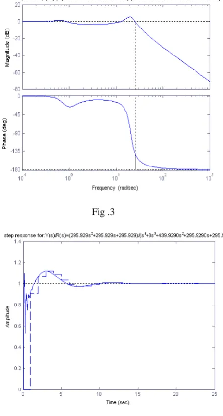
--- s^4 + 8 s^3 + 439.9 s^2 + 295.9 s + 295.9 Gm = Inf Pm = 38.8462
Wcg = Inf Wcp = 25.7402
Margins = Inf Inf 38.8462 25.7402 Transfer function:
295.9 s^2 + 295.9 s + 295.9
---
Transfer function:
0.9056 z^3 - 0.7764 z^2 + 0.3399 z + 0.002744 --- z^4 - 1.038 z^3 + 0.5074 z^2 + 0.001818 z + 0.0003355 Sampling time: 1
d = 1.0000 -1.0380 0.5074 0.0018 0.0003 e = 0.5214 + 0.4898i
0.5214 - 0.4898i -0.0024 + 0.0255i -0.0024 - 0.0255i
s = 0.0003 0.0018 0.5074 -1.0380 1.0000 1.0000 -1.0380 0.5074 0.0018 0.0003 -1.0000 1.0380 -0.5074 -0.0022 0 -0.0022 -0.5074 1.0380 1.0380 0 1.0000 -1.0391 0.5096 0 0 a0 = 3.3550e-004
a4 = 1 b0 = 1.0000 b3 = 0.0022 c0 = 1.0000 c2 = 0.5096
VII. RESULT
• GAIN MARGIN = Inf dB, very high. • PHASE MARGIN= 38.8462deg.
• Rank of the controllability and observability matrix=4, As same as the order of the system and hence controllable and observable.
• Since a4>a0 b3<b0 and c2<c0 so system is stable in sample data control system.
Fig .3
Fig.4
IX. CONCLUSION
Since the system is stable in both continuous and sample data control system, controllable, observable and having appropriate gain and phase margin so the design of an artificial control of standing and leg articulation system becomes feasible.
REFERENCES
[1]. R.C .Dorf, Bishop, “Modern Control System”, 8th ed, Addison
Wesley, 1999, pp-747-747.
[2]. Move de Panne, “A controller for the dynamic walk of a Biped,” Proceedings of the conference on Decision and Control, IEEE, December 1992, pp.2668-2673.
[3]. A.C.Guyton, “Text Book of Medical Physiology”, 6th ed,
W.B.Saunders Company 1981, pp-136.
[4]. Aguayo, A.J. and Karpati, G. (eds): “Current topics in nerves and Muscle Research,” Newyork, Elsevier/North, Holland, 1979. [5]. Winter .D.A.: “Biomechanics of human movement”, Nework,
Jhon Wiley and Sons, 1979.
[6]. Achintya Das, “Advance Control systems”, 2nd ed, Matrix
Educare, February 2008, pp. 286-287.
[7]. Stefani, Shahian, Savant, Hostetter, “Design of feedback Control Systems”,4th ed, Oxford University Press, 2002, pp. 210- 211.
[image:5.595.63.291.73.497.2]