Dual Decomposition Inference for Graphical Models over Strings
∗ Nanyun Peng and Ryan Cotterell and Jason EisnerDepartment of Computer Science, Johns Hopkins University {npeng1,ryan.cotterell,eisner}@jhu.edu
Abstract
We investigate dual decomposition for joint MAP inference of many strings. Given an arbitrary graphical model, we de-compose it into small acyclic sub-models, whose MAP configurations can be found by finite-state composition and dynamic programming. We force the solutions of these subproblems to agree on overlap-ping variables, by tuning Lagrange multi-pliers for an adaptively expanding set of variable-lengthn-gram count features. This is the first inference method for ar-bitrary graphical models over strings that does not require approximations such as random sampling, message simplification, or a bound on string length.Provided that
the inference method terminates, it gives a certificate of global optimality (though MAP inference in our setting is undecid-able in general). On our global phonolog-ical inference problems, it always termi-nates, and achieves more accurate results than max-product and sum-product loopy belief propagation.
1 Introduction
Graphical models allow expert modeling of com-plex relations and interactions between random variables. Since a graphical model with given pa-rameters defines a probability distribution, it can be used to reconstruct values for unobserved vari-ables. Themarginal inferenceproblem is to com-pute the posterior marginal distributions of these variables. The MAP inference (or MPE) prob-lem is to compute the single highest-probability joint assignment to all the unobserved variables.
Inference in general graphical models is NP-hard even when the variables’ values are finite dis-crete values such as categories, tags or domains. In this paper, we address the more challenging setting
∗This material is based upon work supported by the Na-tional Science Foundation under Grant No. 1423276.
where the variables in the graphical models range over strings. Thus, the domain of the variables is aninfinitespace of discrete structures.
In NLP, such graphical models can deal with large, incompletely observed lexicons. They could be used to model diverse relationships among strings that represent spellings or pronunciations; morphemes, words, phrases (such as named enti-ties and URLs), or utterances; standard or variant forms; clean or noisy forms; contemporary or his-torical forms; underlying or surface forms; source or target language forms. Such relationships arise in domains such as morphology, phonology, his-torical linguistics, translation between related lan-guages, and social media text analysis.
In this paper, we assume a given graphical model, whose factors evaluate the relationships among observed and unobserved strings.1 We
present a dual decomposition algorithm for MAP inference, which returns a certifiably optimal so-lution when it converges. We demonstrate our method on a graphical model for phonology pro-posed by Cotterell et al. (2015). We show that the method generally converges and that it achieves better results than alternatives.
The rest of the paper is arranged as follows: We will review graphical models over strings in sec-tion 2, and briefly introduce our sample problem in section 3. Section 4 develops dual decompo-sition inference for graphical models over strings. Then our experimental setup and results are pre-sented in sections 5 and 6, with some discussion.
2 Graphical Models Over Strings
2.1 Factor Graphs and MAP Inference
To perform inference on a graphical model (di-rected or undi(di-rected), one first converts the model to a factor graph representation (Kschischang et al., 2001). A factor graph is a finite bipartite
1In some task settings, it is also necessary to discover the
model topology along with the model parameters. In this pa-per we do not treat that structure learning problem. However, both structure learning and parameter learning need to call inference—such as the method presented here—in order to evaluate proposed topologies or improve their parameters.
z
rizajgn eɪʃən dæmn
rεzɪgn#eɪʃən rizajn#z dæmn#z dæmn#eɪʃən
r,εzɪgn’eɪʃn riz’ajnz d’æmz d,æmn’eɪʃn
resignation resigns damns damnation
1) Underlying morphemes
Concatenation
2) Underlying words
Phonology
[image:2.595.78.524.66.181.2]3) Surface words
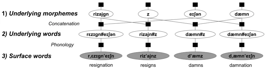
Figure 1: A fragment of the factor graph for the directed graphical model of Cotterell et al. (2015), displaying a possible assignment to the variables (ellipses). The model explains each observed surface word as the result of applying phonology to a concatenation of underlying morphemes. Shaded variables show the observed surface forms for four words:resignation,
resigns,damns, anddamnation. The underlying pronunciations of these words are assumed to be more similar than their surface pronunciations, because the words are known to share latent morphemes. The factor graph encodes what is shared. Each observed word at layer 3 has a latent underlying form at layer 2, which is a deterministic concatenation of latent morphemes at layer 1. The binary factors between layers 2 and 3 score each (underlying,surface) pair for its phonological plausibility. The unary factors at layer 1 score each morpheme for its lexical plausibility. See Cotterell et al. (2015) for discussion of alternatives.
graph over a set X = {X1, X2, . . .} of variables
and a setF of factors. Anassignmentto the vari-ables is a vector of valuesx= (x1, x2, . . .). Each
factorF ∈ F is a real-valued function ofx, but it depends on a givenxionly ifF is connected toXi
in the graph. Thus, a degreed-factor scores some length-d subtuple of x. The score of the whole joint assignment simply sums over all factors:
score(x)=def X
F∈F
F(x). (1)
We seek the x of maximum score that is con-sistent with our partial observation of x. This is a generic constraint satisfaction problem with soft constraints. While our algorithm does not de-pend on a probabilistic interpretation of the fac-tor graph,2 it can be regarded as peforming
max-imum a posteriori(MAP) inference of the unob-served variables, under the probability distribution p(x)= (1def /Z) expscore(x).
2.2 The String Case
Graphical models over strings have enjoyed some attention in the NLP community. Tree-shaped graphical models naturally model the evolution-ary tree of word forms (Bouchard-Cˆot´e et al., 2007; Bouchard-Cˆot´e et al., 2008; Hall and Klein, 2010; Hall and Klein, 2011). Cyclic graphical
2E.g., it could be used for exactly computing the
separa-tion oracle when training a structural SVM (Tsochantaridis et al., 2005; Finley and Joachims, 2007). Another use is mini-mum Bayes risk decoding—computing the joint assignment having minimum expected loss—if the loss function does not decompose over the variables, but a factor graph can be con-structed that evaluates the expected loss of any assignment.
models have been used to model morphological paradigms (Dreyer and Eisner, 2009; Dreyer and Eisner, 2011) and to reconstruct phonological un-derlying forms of words (Cotterell et al., 2015).
The variables in such a model are strings of un-bounded length: each variableXi is permitted to
range over Σ∗ where Σ is some fixed, finite
al-phabet. As in previous work, we assume that a degree-d factor is a d-way rational relation, i.e., a function of d strings that can be computed by ad-tapeweighted finite-state machine (WFSM)
(Mohri et al., 2002; Kempe et al., 2004). Such a machine is called anacceptor (WFSA) ifd = 1 or atransducer (WFST)ifd= 2.3
Past work has shown how to approximately
sample from the distribution over x defined by such a model (Bouchard-Cˆot´e et al., 2007), or ap-proximately compute the distribution’smarginals
using variants of sum-product belief propaga-tion(BP) (Dreyer and Eisner, 2009) and expecta-tion propagaexpecta-tion (EP) (Cotterell and Eisner, 2015).
2.3 Finite-State Belief Propagation
BP iteratively updates messages between factors and variables. Each message is a vector whose el-ements score the possible values of a variable.
Murphy et al. (1999) discusses BP on cyclic (“loopy”) graphs. For pedagogical reasons, sup-pose momentarily that all factors have degree≤2 (this loses no power). Then BP manipulates only vectors and matrices—whose dimensionality de-pends on the number of possible values of the
vari-3Finite-state software libraries often support only these
ables. In the string case, they haveinfinitelymany rows and columns, indexed by possible strings.
Dreyer and Eisner (2009) represented these in-finite vectors and matrices by WFSAs and WF-STs, respectively. They observed that the simple linear-algebra operations used by BP can be im-plemented by finite-state constructions. The point-wise product of two vectors is the intersection of their WFSAs; the marginalization of a matrix is the projection of its WFST; a vector-matrix prod-uct is computed by composing the WFSA with the WFST and then projecting onto the output tape. For degree > 2, BP’s rank-d tensors become d -tape WFSMs, and these constructions generalize.
Unfortunately, except in small acyclic models, the BP messages—which are WFSAs—usually become impractically large. Each intersection or composition involves a cross-product construc-tion. For example, when finding the marginal distribution at a degree-dvariable, intersecting d WFSA messages havingmstates each may yield a WFSA with up to md states. (Our models in
section 6 include variables with d up to 156.) Combiningmanycross products, as BP iteratively passes messages along a path in the factor graph, leads to blowup that is exponential in the length of the path—which in turn is unbounded if the graph has cycles (Dreyer and Eisner, 2009), as ours do.
The usual solution is to prune or otherwise ap-proximate the messages at each step. In particu-lar, Cotterell and Eisner (2015) gave a principled way to approximate the messages using variable-length n-gram models, using an adaptive variant of Expectation Propagation (Minka, 2001).
2.4 Dual Decomposition Inference
In section 4, we will present a dual decomposition (DD) method that decomposes the original com-plex problem into many small subproblems that are free of cycles and high degree nodes. BP can solve each subproblem without approximation.4
The subproblems “communicate” through La-grange multipliers that guide them towards agree-ment on a single global solution. This information is encoded in WFSAs that score possible values of a string variable. DD incrementally adjusts the WFSAs so as to encourage values that agree with
4Such small BP problems commonly arise in NLP. In
par-ticular, using finite-state methods to decode a composition of several finite-state noisy channels (Pereira and Riley, 1997; Knight and Graehl, 1998) can be regarded as BP on a graph-ical model over strings that has a linear-chain topology.
the variable’s average value across subproblems. Unlike BP messages, the WFSAs in our DD method will be restricted to be variable-length n-gram models, similar to Cotterell and Eisner (2015). They may still grow over time; but DD of-ten halts while the WFSAs are still small. It halts when its strings agree exactly, rather than when it has converged up to a numerical tolerance, like BP.
2.5 Switching Between Semirings
Our factors may benondeterministicWFSMs. So whenF ∈ F scores a givend-tuple of string val-ues, it may accept thatd-tuple along multiple dif-ferent WFSM paths with difdif-ferent scores, corre-sponding to different alignments of the strings.
For purposes of MAP inference, we defineF to return themaximumof these path scores. That is, we take the WFSMs to be defined with weights in the (max,+) semiring (Mohri et al., 2002). Equivalently, we are seeking the “best global solu-tion” in the sense of choosing not only the strings xibut also the alignments of thed-tuples.5
To do so, we must solve each DD subprob-lem in the same sense. We usemax-product BP. This still applies the Dreyer-Eisner method of sec-tion 2.3. Since these WFSMs are defined in the (max,+)semiring, the method’s finite-state oper-ations will combine weights usingmaxand+.
MAP inference in our setting is in general com-putationally undecidable.6 However, if DD
con-verges (as in our experiments), thenits solution is guaranteed to be the true MAP assignment.
In section 6, we will compare DD with (loopy) max-product BP and (loopy) sum-product BP. These respectively approximate MAP inference and marginal inference over the entire factor graph. Marginal inference computes marginal string probabilities that sum (rather than maxi-mize) over the choices of other strings and the choices of paths. Thus, for sum-product BP, we re-interpret the factor WFSMs as defined over the (logadd,+) semiring. This means that the expo-nentiated score assigned by a WFSM is the sum of the exponentiated scores of the accepting paths.
5This problem is more specifically calledMPE inference. 6The trouble is that we cannot bound the length of the
r,εzɪgn’eɪʃn riz’ajnz d,æmn’eɪʃn d’æmz
Subproblem 1 Subproblem 2 Subproblem 3 Subproblem 4
z rizajn
eɪʃən dæmn eɪʃən dæmn z
rεzɪgn
[image:4.595.78.289.66.143.2]rεzɪgn#eɪʃən rizajn#z dæmn#eɪʃən dæmn#z
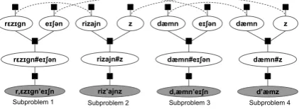
Figure 2: To apply dual decomposition, we choose to decom-pose 1 into one subproblem per surface word. Dashed lines connect two or more variables from different subproblems that correspond to the same variable in the original graph. The method of Lagrange multipliers is used to force these variables to have identical values. An additional unary factor attached to each subproblem variable (not shown) is used to incorporate its Lagrangian term.
3 A Sample Task: Generative Phonology
Before giving the formal details of our DD method, we give a motivating example: a recently proposed graphical model for morphophonology. Cotterell et al. (2015) defined a Bayesian network to describe the generative process of phonological words. Our Figure 1 shows a conversion of their model to a factor graph and explains what the vari-ables and factors mean.
Inference on this graph performs unsupervised discovery of latent strings. Given observed surface representations of words (SRs), inference aims to recover the underlying representations (URs) of the words and their shared constituent morphemes. The latter can then be used to predict held-out SRs. Notice that the 8 edges in the first layer of Fig-ure 1 form a cycle; such cycles make BP inexact. Moreover, the figure shows only a schematic frag-ment of the graphical model. In the actual exper-iments, the graphical models have up to 829 vari-ables, and the variables representing morpheme URs are connected to up to 156 factors (because many words share the same affix).
To handle the above challenges without ap-proximation, we want to decompose the original problem into subproblems where each subproblem can be solved efficiently. In particular, we want the subproblems to be free of cycles and high-degree nodes. In our phonology example, each observed word along with its correspondent latent URs forms an ideal subproblem. This decomposi-tion is shown in Figure 2.
While the subproblems can be solved efficiently in isolation, they may share variables, as shown by the dashed lines in Figure 2. DD repeatedly modifies and re-solves the subproblems until they agree on their shared variables.
4 Dual Decomposition
Dual decomposition is a general technique for solving constrained optimization problems. It has been widely used for MAP inference in graphi-cal models (Komodakis et al., 2007; Komodakis and Paragios, 2009; Koo et al., 2010; Martins et al., 2011; Sontag et al., 2011; Rush and Collins, 2014). However, previous work has focused on variablesXi whose values are inRor a small
fi-nite set; we will consider the infifi-nite setΣ∗.
4.1 Review of Dual Decomposition
To apply dual decomposition, we must partition the original problem into a union ofK subprob-lems, each of which can be solved exactly and ef-ficiently (and in parallel). For example, our exper-iments partition Figure 1 as shown in Figure 2.
Specifically, we partition the factors intoKsets
F1, . . . ,FK. Each factor F ∈ F appears in
ex-actly one of these sets. This lets us rewrite the score (1) asPkPF∈FkF(x). Instead of simply
seeking its maximizerx, we equivalently seek
argmax
x1,...,xK K X
k=1 X
F∈Fk
F(xk)s.t.x1=· · ·=xK
(2)
If we dropped the equality constraint, (2) could be solved by separately maximizing
P
F∈FkF(xk)for each k. This “subproblem” is
itself a MAP problem which considers only the factorsFk and the variablesXk adjacent to them
in the original factor graph. The subproblem ob-jective does not depend on the other variables.
We now attempt to enforce the equality con-straint indirectly, by adding Lagrange multipli-ers that encourage agreement among the subprob-lems. Assume for the moment that the variables in the factor graph are real-valued (eachxk
i is inR).
Then consider theLagrangian relaxationof (2),
max
x1,...,xK K X
k=1 X
F∈Fk
F(xk) +X
i
λki ·xki (3)
This can still be solved by separate maximizations. Foranychoices ofλk
i ∈ Rhaving(∀i)Pkλki =
0, it upper-bounds the objective of (2). Why? The solution to (2) achieves the same value in (3), yet (3) may do even better by considering solutions that do not satisfy the constraint. Our goal is to find λk
i values that tighten this upper bound as
much as possible. Ifwe can findλk
the optimum of (3) satisfies the equality constraint, then we have a tight bound and a solution to (2).
To improve the method, recall that subproblem kconsiders only variablesXk. It is indifferent to
the value ofXiifXi ∈ X/ k, so we just leavexki
un-defined in the subproblem’s solution. We treat that as automatically satisfying the equality constraint; thus we do not need any Lagrange multiplierλk
i to
force equality. Our final solutionxignores unde-fined values, and setsxito the value agreed on by
the subproblems thatdidconsiderXi.7
4.2 Substring Count Features
But what do we do if the variables are strings? The Lagrangian termλk
i·xki in (3) is now ill-typed. We
replace it with λk
i ·γ(xki), whereγ(·) extracts a
real-valued feature vectorfrom a string, andλk i
is a vector of Lagrange multipliers.
This corresponds to changing the constraint in (2). Instead of requiringx1
i = · · ·=xKi for each
i, we are now requiringγ(x1
i) = · · · = γ(xKi ),
i.e., these strings must agreein their features. We want each possible string to have a unique feature vector, so that matching features forces the actual strings to match. We follow Paul and Eisner (2012) and use asubstring count featurefor each w∈Σ∗. In other words,γ(x)is an infinitely long
vector, which maps eachwto the number of times thatwappears inxas a substring.8
Computing λk
i ·γ(xki) in (3) remains
possi-ble because in practice,λk
i will have only finitely
many nonzeros. This is so because our feature vector γ(x) has only finitely many nonzeros for any stringx, and the subgradient algorithm in sec-tion 4.3 below always updatesλk
i by adding
mul-tiples of suchγ(x)vectors.
We will use a further trick below to prevent rapid growth of this finite set of nonzeros. Each variable Xi maintains an active set of features,
Wi. Only these features may have nonzero
La-grange multipliers. While the active set can grow over time, it will be finite at any given step.
Given the Lagrange multipliers, subproblem k of (3) is simply MAP inference on the factor graph consisting of the variablesXk and factorsFk as well asan extra unary factorGk
i at eachXi ∈ Xk: 7Without this optimization, the Lagrangian termλk
i ·xki would have drivenxk
i to match that value anyway.
8More precisely, the number of times thatwappears in
BOSxEOS, whereBOS,EOSare distinguished boundary sym-bols. We allow wto start withBOS and/or end withEOS, which yields prefix and suffix indicator features.
Gk
i(xk)=defλik·γ(xki) (4)
These unary factors penalize strings according to the Lagrange multipliers. They can be encoded as WFSAs (Allauzen et al., 2003; Cotterell and Eisner, 2015, Appendices B.1–B.5), allowing us to solve the subproblem by max-product BP as usual. The topology of the WFSA forGk
i depends only
onWi, while its weights come fromλki. 4.3 Projected Subgradient Method
We aim to adjust the collection λ of Lagrange multipliers tominimizethe upper bound (3). Fol-lowing Komodakis et al. (2007), we solve this con-vex dual problem using a projected subgradient method. We initializeλ = 0and compute (3) by solving theK subproblems. Then we take a step to adjustλ, and repeat in hopes of eventually sat-isfying the equality condition.
The projected subgradient step is
λki :=λki +η·µi−γ(xki)
(5)
whereη >0is the current step size, andµi is the
mean ofγ(xk0
i )over all subproblemsk0 that
con-siderXi. This update modifies (3) to encourage
solutionsxksuch thatγ(xk
i)comes closer toµi. For eachi,we update allλk
i at once to preserve
the property that(∀i)Pkλk
i = 0. However, we
are only allowed to update components of theλk i
that correspond to features in the active setWi. To
ensure that we continue to make progress even af-ter we agree on these features, we first expandWi
by adding theminimalstrings (if any) on which the xk
i do not yet all agree. For example, we will add
theabcfeature only when thexki already agree on
their counts of its substringsabandbc.9
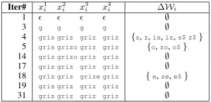
Algorithm 1 summarizes the whole method. Ta-ble 1 illustrates how one active setWi(section 4.3)
evolves, in our experiments, as it tries to enforce agreement on a particular stringxi.
4.4 Past Work: Implicit Intersection
Our DD algorithm is an extension of one that Paul and Eisner (2012) developed for the simpler im-plicit intersectionproblem. Given many WFSAs F1, . . . , FK, they were able to find the string x
with maximum total scorePKk=1Fk(x). (They
ap-plied this to solve instances of the NP-hardSteiner
9In principle, we should check that they also (still) agree
Algorithm 1DD for graphical models over strings
1: initialize the active setWifor each variableXi∈ X 2: initializeλki =0for eachXiand each subproblemk 3: fort= 1 toT do .max number of iterations 4: fork= 1 toKdo .solve all primal subproblems 5: ifany of theλki have changedthen
6: run max-product BP on the acyclic graph de-fined by variablesXkand factorsFkandGk i 7: extract MAP strings: ∀iwithXi ∈ Xk,xki is the label of the max-scoring accepting path in the WFSA that represents the belief atXi 8: foreachXi∈ Xdo .improve dual bound 9: ifthe defined stringsxk
i are not all equalthen 10: Expand active feature setWi .section 4.3
11: Update eachλki .equation (5)
12: Update eachGk
i fromΘi,λki .see (4) 13: ifnone of theXirequired updatesthen
14: returnany definedxk
i (all are equal) for eachi 15: return{x1
i, . . . , xKi }for eachi .failed to converge
stringproblem, i.e., finding the string xof mini-mum total edit distance to a collection ofK ≈100 given strings.) The naive solution to this problem would be to find the highest-weighted path in the intersectionF1∩ · · · ∩FK. Unfortunately, the
in-tersection of WFSAs takes the Cartesian product of their state sets. Thus materializing this inter-section would have taken time exponential inK.
To put this another way, inference is NP-hard even on a “trivial” factor graph: asinglevariable X1attached toKfactors. Recall from section 2.3
that BP would solve this via the expensive inter-section above. Paul and Eisner (2012) instead ap-plied DD with one subproblem per factor. We generalize their method to handle arbitrary factor graphs, with multiple latent variables and cycles.
4.5 Block Coordinate Update
We also explored a possible speedup for our algo-rithm. We used ablock coordinate update vari-ant of the algorithm when performing inference on the phonology problem and observed an empiri-cal speedup. Block coordinate updates are widely used in Lagrangian relaxation and have also been explored specifically for dual decomposition.
In general, block algorithms minimize the ob-jective by holding some variables fixed while up-dating others. Sontag et al. (2011) proposed a so-phisticated block method called MPLP that con-siders all values of variableXiinstead of the ones
obtained from the best assignments for the sub-problems. However, it is not clear how to apply their technique to string-valued variables. Instead, the algorithm we propose here is much simpler—it
Iter# x1
i x2i x3i x4i ∆Wi
1 ∅
3 g g g g ∅
4 gris griz griz griz {s,z,is,iz,s$ z$}
5 gris grizo griz griz {o,zo,o$}
14 griz grizo griz griz ∅
17 griz griz griz griz ∅
18 griz griz grize griz {e,ze,e$}
19 gris griz griz griz ∅
[image:6.595.309.524.61.165.2]31 griz griz griz griz ∅
Table 1: One variable’s active set as DD runs. This variable is the unobserved stem morpheme shared by the Catalan words gris, grizos, grize, grizes. The second column shows the current set of solutions from the 4 subproblems having copies of this variable. The third column shows the new sub-strings that are then added to the active set, to try to enforce agreement via their Lagrange multipliers. The table does not show iterations in which these columns have not changed. However, those iterations still update the Lagrange multipli-ers to more strongly encourage agreement (if needed). Al-though agreement is achieved at iterations 1, 3, and 17, it is then disrupted—the subproblems’ solutions change be-cause of Lagrange-multiplier pressures on theirother vari-ables (suffixes that donotagree yet). At iteration 31, the vari-able returns to agreement ongriz, and never changes again.
divides the primal variables into groups and up-dates each group’s associated dual variables in turn, using a single subgradient step (5). Note that this way of partitioning the dual variables has the nice property that we can still use the projected subgradient update we gave in (5) and preserve the property that(∀i)Pkλk
i = 0.
In the graphical model for generative phonol-ogy, there are two types of underlying morphemes in the first layer: word stems and word affixes. Our block coordinate update algorithm thus alternates between subgradient updates to the dual variables for the stems and the dual variables for the affixes. Note that when performing block coordinate up-date on the dual variables, the primal variables are
not held constant, but rather are chosen by opti-mizing the corresponding subproblem.
5 Experimental Setup
5.1 Datasets
We compare DD to belief propagation, using the graphical model for generative phonology dis-cussed in section 3. Inference in this model aims to reconstruct underlying morphemes. Since our fo-cus is inference, we will evaluate these reconstruc-tions directly (whereas Cotterell et al. (2015) eval-uated their ability to predict novel surface forms using the reconstructions).
How-ever, they are actually derived from datasets con-structed by Cotterell et al. (2015), which are avail-able with full descriptions athttp://hubal.cs. jhu.edu/tacl2015/. Briefly:
EXERCISE Small datasets of Catalan, English,
Maori, and Tangale, drawn from phonology textbooks. Each dataset contains 55 to 106 surface words, formed from a collection of 16 to 55 morphemes.
CELEX Larger datasets of German, English, and Dutch, drawn from the CELEX database (Baayen et al., 1995). Each dataset contains 1000 surface words, formed from 341 to 381 underlying morphemes.
5.2 Evaluation Scheme
We compared three types of inference:
DD Use DD to performexact MAP inference.
SP Perform approximate marginal inference by sum-product loopy BP with pruning (Cot-terell et al., 2015).
MP Perform approximate MAP inference by max-product loopy BP with pruning. DD and SP improve this baseline in different ways.
DD predicts a string value for each variable. For SP and MP, we deem the prediction at a variable to be the string that is scored most highly by the belief at that variable.
We report the fraction of predicted morpheme URs that exactly match the gold-standard URs proposed by a human (Cotterell et al., 2015). We also compare these predicted URs to one another, to see how well the methods agree.
5.3 Parameterization
The model of Cotterell et al. (2015) has two fac-tor types whose parameters must be chosen.10
The first is a unary factorMφ. Each
underlying-morpheme variable (layer 1 of Figure 1) is con-nected to a copy ofMφ, which gives the prior
dis-tribution over its values. The second is a binary factorSθ. For each surface word (layer 3), a copy
of Sθ gives its conditional distribution given the
corresponding underlying word (layer 2).Mφand
Sθrespectively model thelexiconand the phonol-ogyof the specific language; both are encoded as WFSMs.
10The model also has a three-way factor, connecting layers
1 and 2 of Figure 1. This represents deterministic concatena-tion (appropriate for these languages) and has no parameters.
Mφis a 0-gram generative model: at each step
it emits a character chosen uniformly from the al-phabetΣwith probabilityφ, or halts with proba-bility1−φ. It favors shorter strings in general, but φdetermines how weak this preference is.
Sθ is a sequential edit model that produces a
word’s SR by stochastically copying, inserting, substituting, and deleting the phonemes of its UR. We explore two ways of parameterizing it.
Model 1is a simple model in whichθis a scalar, specifying the probability of copying the next character of the underlying word as it is transduced to the surface word. The remaining probability mass1−θis apportioned equally among insertion, substitution and deletion operations.11 This
mod-els phonology as “noisy concatenation”—the min-imum necessary to account for the fact that surface words cannot quite be obtained as simple concate-nations of their shared underlying morphemes.
Model 2 is a replication of the much more complicated parametric model of Cotterell et al. (2015), which can handle linguistic phonology. Here the factorSθ is acontextual edit FST
(Cot-terell et al., 2014). The probabilities of competing edits in a given context are determined by a log-linear model with weight vectorθand features that are meant to pick up on phonological phenomena.
5.4 Training
When evaluating an inference method from sec-tion 5.2, we use the same inference method both for prediction and within training.
We train Model 1 by grid search. Specifically, we choose φ ∈ [0.65,1) andθ ∈ [0.25,1)such that the predicted forms maximize the joint score (1) (always using the(max,+)semiring).
For Model 2, we compared two methods for training theφandθparameters (θis a vector):
Model 2S Supervised training, which observes
the “true” (hand-constructed) values of the URs. This idealized setting uses the best pos-sible parameters (trained on the test data).
Model 2E Expectation maximization (EM), whose E stepimputesthe unobserved URs. EM’s E step calls forexact marginal inference, which is intractable for our model. So we substi-tute the same inference method that we are
test-11That is, probability mass of(1−θ)/3is divided equally
ing. This gives us three approximations to EM, based on DD, SP and MP. Note that DD specif-ically gives the Viterbi approximation to EM— which sometimes gets better results than true EM (Spitkovsky et al., 2010). For MP (but not SP), we extract only the 1-best predictions for the E step, since we study MP as an approximation to DD.
As initialization, our first E step uses the trained version of Model 1 for the same inference method.
5.5 Inference Details
We run SP and MP for 20 iterations (usually the predictions converge within 10 iterations). We run DD to convergence (usually<600iterations). DD iterations are much faster since each variable con-siders d strings, not d distributions over strings. Hence DD does not intersect distributions, and many parts of the graph settle down early because discrete values can converge in finite time.12
We follow Paul and Eisner (2012, section 5.1) fairly closely. In particular: Our stepsize in (5) is
η = α/(t+ 500), where t is the iteration
num-ber; α = 1for Model 2S andα = 10 otherwise. We proactively include all 1-gram and 2-gram sub-string features in the active sets Wi at
initializa-tion, rather than adding them only as needed. At it-erations 200, 400, and 600, we proactively add all 3-, 4-, and 5-gram features (respectively) on which the counts still disagree; this accelerates conver-gence on the few variables that have not already converged. We handle negative-weight cycles as Paul and Eisner do. If we had ever failed to con-verge within 2000 iterations, we would have used their heuristic to extract a prediction anyway.
Model 1 suffers from a symmetry-breaking problem. Many edits have identical probability, and when we run inference, many assignments will tie for highest scoring configuration. This can prevent DD from converging and makes per-formance hard to measure. To break these ties, we add “jitter” separately to each copy of Mφ
in Figure 1. Specifically, if Fi is the unary
fac-tor attached to Xi, we expand our 0-gram model
Fi(x) = log((p/|Σ|)|x| · (1 − p)) to become
Fi(x) = log(Qc∈Σpc,i|x|c ·(1 −p)), where |x|c
denotes the count of character c in string x, and pc,i ∝ (p/|Σ|)·expεc,i whereεc,i ∼N(0,0.01)
and we preservePc∈Σpc,i =p.
12A variable need not updateλif its strings agree; a
sub-problem is not re-solved if none of its variables updatedλ.
(a) Tangale (b) Catalan
[image:8.595.309.538.62.258.2](c) Maori (d) English
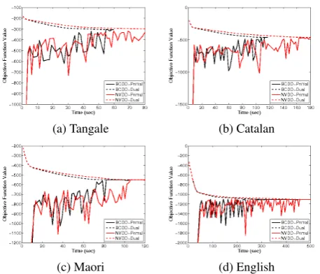
Figure 3: The primal-dual curve of NVDD v.s. BCDD on 4 EXERCISElanguages. BCDD always converges faster.
6 Experimental Results
6.1 Convergence and Speed of DD
As linguists know, reconstructing an underlying stem or suffix can be difficult. We may face insuf-ficient evidence or linguistic irregularity—or reg-ularity that goes unrecognized because the phono-logical model is impoverished (Model 1) or poorly trained (early EM iterations on Model 2). DD may then require extensive negotiation to resolve disagreements among subproblems. Furthermore, DD must renegotiate as conditions change else-where in the factor graph (Table 1).
DD converged in all of our experiments. Note that DD (section 4.3) has converged when all the equality constraints in (2) are satisfied. In this case, we have found the true MAP configuration.
In section 4.5, we discussed a block coordi-nate update variation (BCDD) of our DD algo-rithm. Figure 3 shows the convergence behavior of BCDD against the naive projected subgradi-ent algorithm (NVDD) on the four EXERCISE
lan-guages under Model 1. The dual objective (3) al-ways upper-bounds the primal score (i.e., the score (1) of an assignment derived heuristically from the current subproblem solutions). The dual de-creases as the algorithm progresses. When the two objectives meet, we have found an optimal solu-tion to the primal problem. We can see in Figure 3 that our DD algorithm converges quickly on the four EXERCISE languages and BCDD converges
consistently faster than NVDD. We use BCDD in the remaining experiments.
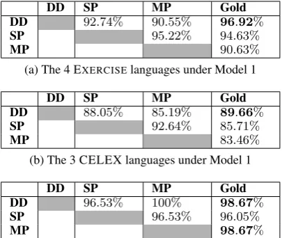
DD SP MP Gold DD 92.74% 90.55% 96.92%
SP 95.22% 94.63%
MP 90.63%
(a) The 4 EXERCISElanguages under Model 1
DD SP MP Gold DD 88.05% 85.19% 89.66%
SP 92.64% 85.71%
MP 83.46%
(b) The 3 CELEX languages under Model 1
DD SP MP Gold
DD 96.53% 100% 98.67%
SP 96.53% 96.05%
MP 98.67% (c) The 3 CELEX languages under Model 2S (EXERCISE
dataset gives 100% everywhere)
DD SP MP Gold DD 92.43% 89.39% 98.18%
SP 96.73% 95.42%
MP 90.74%
[image:9.595.80.283.72.243.2](d) The 4 EXERCISElanguages under Model 2E Table 2: Pairwise agreement (on morpheme URs) of DD, SP, MP and the gold standard, for each group of inference prob-lems. Boldface is highest accuracy (agreement with gold).
other methods. It is typically faster on the EXER -CISEdata, and a few times slower on the CELEX
data. But we stop the other methods after 20 it-erations, whereas DD runs until it gets an exact answer. We find that this runtime is unpredictable and sometimes quite long. In the grid search for training Model 1, we observed that changes in the parameters(φ, θ)could cause the runtime of DD inference to vary by 2 orders of magnitude. Sim-ilarly, on the CELEX data, the runtime on Model 1 (over 10 differentN = 600subsets of English) varied from about 1 hour to nearly 2 days.13
6.2 Comparison of Inference
For each language, we constructed several differ-ent unsupervised prediction problems. In each problem, we observe some size-N subset of the words in our dataset, and we attempt to predict the URs of the morphemes in those words. For each CELEX language, we took N = 600, and used three of the size-N training sets from (Cotterell et al., 2015). For each EXERCISE language, we
took N to be one less than the dataset size, and used allN + 1subsets of sizeN, again similar to (Cotterell et al., 2015). We report the unweighted macro-average of all these accuracy numbers.
13Note that our implementation is not optimized; e.g., it
uses Python (not Cython).
We compare DD, SP, and MP inference on each language under different settings. Table 2 shows aggregate results, as an unweighted aver-age over multiple languaver-ages and training sets. We present various additional results at http://cs. jhu.edu/˜npeng/emnlp2015/, including a per-language breakdown of the results, runtime num-bers, and significance tests.
The results for Model 1 are shown in Tables 2a and 2b. As we can see, in both datasets, dual decomposition performed the best at recovering the URs, while MP performed the worst. Both DD and MP are doing MAP inference, so the dif-ferences reflect the search error in MP. Interest-ingly, DD agrees more with SP than with MP, even though SP uses marginal inference.
Although the aggregate results on the EXER -CISE dataset show a large improvement of DD
over both of the BP algorithms, the gain all comes from the English language. SP actually does better than DD on Catalan and Maori, and MP also gets better results than DD on Maori, tying with SP.
For Model 2S, all inference methods achieved 100% accuracy on the EXERCISE dataset, so we
do not show a table. The results on the CELEX dataset are shown in Table 2c. Here both DD and MP performed equally well, and outperformed BP—a result like (Spitkovsky et al., 2010). This trend is consistent over all three languages: DD and MP always achieve similar results and both outperform SP. Of course, one advantage of DD in the setting is that it actually finds the true MAP prediction of the model; the errors are known to be due to the model, not the search procedure.
For Model 2E, we show results on the EXER -CISEdataset in Table 2d. Here the results resemble
the pattern of Model 1.
7 Conclusion and Future Work
We presented a general dual decomposition algo-rithm for MAP inference on graphical models over strings, and applied it to an unsupervised learn-ing task in phonology. The experiments show that our DD algorithm converges and gets better results than both max-product and sum-product BP.
References
Cyril Allauzen, Mehryar Mohri, and Brian Roark. 2003. Generalized algorithms for constructing sta-tistical language models. In Proceedings of ACL, pages 40–47.
R. Harald Baayen, Richard Piepenbrock, and Leon Gu-likers. 1995. The CELEX lexical database on CD-ROM.
Alexandre Bouchard-Cˆot´e, Percy Liang, Thomas L Griffiths, and Dan Klein. 2007. A probabilistic ap-proach to diachronic phonology. InProceedings of EMNLP-CoNLL, pages 887–896.
Alexandre Bouchard-Cˆot´e, Percy Liang, Thomas Grif-fiths, and Dan Klein. 2008. A probabilistic ap-proach to language change. InProceedings of NIPS.
Ryan Cotterell and Jason Eisner. 2015. Penalized expectation propagation for graphical models over strings. InProceedings of NAACL-HLT, pages 932– 942, Denver, June. Supplementary material (11 pages) also available.
Ryan Cotterell, Nanyun Peng, and Jason Eisner. 2014. Stochastic contextual edit distance and probabilistic FSTs. In Proceedings of ACL, Baltimore, June. 6 pages.
Ryan Cotterell, Nanyun Peng, and Jason Eisner. 2015. Modeling word forms using latent underlying morphs and phonology. Transactions of the Associ-ation for ComputAssoci-ational Linguistics, 3:433–447. Markus Dreyer and Jason Eisner. 2009. Graphical
models over multiple strings. In Proceedings of EMNLP, pages 101–110, Singapore, August.
Markus Dreyer and Jason Eisner. 2011. Discover-ing morphological paradigms from plain text usDiscover-ing a Dirichlet process mixture model. InProceedings of EMNLP, pages 616–627, Edinburgh, July.
Thomas Finley and Thorsten Joachims. 2007. Param-eter learning for loopy markov random fields with structural support vector machines. InICML Work-shop on Constrained Optimization and Structured Output Spaces.
David Hall and Dan Klein. 2010. Finding cognate groups using phylogenies. InProceedings of ACL.
David Hall and Dan Klein. 2011. Large-scale cognate recovery. InProceedings of EMNLP.
Andr´e Kempe, Jean-Marc Champarnaud, and Jason Eisner. 2004. A note on join and auto-intersection of n-ary rational relations. In Loek Cleophas and Bruce Watson, editors, Proceedings of the Eind-hoven FASTAR Days (Computer Science Technical Report 04-40), pages 64–78. Department of Math-ematics and Computer Science, Technische Univer-siteit Eindhoven, Netherlands, December.
Kevin Knight and Jonathan Graehl. 1998. Machine transliteration.Computational Linguistics, 24(4).
Nikos Komodakis and Nikos Paragios. 2009. Beyond pairwise energies: Efficient optimization for higher-order MRFs. InProceedings of CVPR, pages 2985– 2992. IEEE.
Nikos Komodakis, Nikos Paragios, and Georgios Tzir-itas. 2007. MRF optimization via dual decomposi-tion: Message-passing revisited. InProceedings of ICCV, pages 1–8. IEEE.
Terry Koo, Alexander M. Rush, Michael Collins, Tommi Jaakkola, and David Sontag. 2010. Dual decomposition for parsing with non-projective head automata. InProceedings of EMNLP, pages 1288– 1298.
F. R. Kschischang, B. J. Frey, and H. A. Loeliger. 2001. Factor graphs and the sum-product algo-rithm. IEEE Transactions on Information Theory, 47(2):498–519, February.
Andr´e Martins, M´ario Figueiredo, Pedro Aguiar, Eric P. Xing, and Noah A. Smith. 2011. An aug-mented lagrangian approach to constrained map in-ference. InProceedings of ICML, pages 169–176.
Thomas P. Minka. 2001. Expectation propagation for approximate Bayesian inference. InProceedings of UAI, pages 362–369.
Mehryar Mohri, Fernando Pereira, and Michael Ri-ley. 2002. Weighted finite-state transducers in speech recognition. Computer Speech & Language, 16(1):69–88.
Kevin P. Murphy, Yair Weiss, and Michael I. Jordan. 1999. Loopy belief propagation for approximate in-ference: An empirical study. InProceedings of UAI, pages 467–475.
Michael J. Paul and Jason Eisner. 2012. Implicitly in-tersecting weighted automata using dual decompo-sition. InProceedings of NAACL, pages 232–242.
Fernando C. N. Pereira and Michael Riley. 1997. Speech recognition by composition of weighted fi-nite automata. In Emmanuel Roche and Yves Schabes, editors,Finite-State Language Processing. MIT Press, Cambridge, MA.
Alexander M. Rush and Michael Collins. 2014. A tutorial on dual decomposition and Lagrangian re-laxation for inference in natural language process-ing. Technical report available from arXiv.org
asarXiv:1405.5208.
Valentin I. Spitkovsky, Hiyan Alshawi, Daniel Juraf-sky, and Christopher D. Manning. 2010. Viterbi training improves unsupervised dependency parsing. InProceedings of CoNLL, page 917, Uppsala, Swe-den, July.