More Features Are Not Always Better: Evaluating Generalizing Models in Incident Type Classification of Tweets

More Features Are Not Always Better: Evaluating Generalizing Models in

Incident Type Classification of Tweets

Axel Schulz

Business Intelligence Marketing DB Fernverkehr AG

Germany

[email protected]

Christian Guckelsberger Computational Creativity Group Goldsmiths College, University of London

United Kingdom

[email protected]

Benedikt Schmidt

Telecooperation Lab, Technische Universit¨at Darmstadt, Germany

[email protected]

Abstract

Social media represents a rich source of up-to-date information about events such as in-cidents. The sheer amount of available infor-mation makes machine learning approaches a necessity for further processing. This learn-ing problem is often concerned with region-ally restricted datasets such as data from only one city. Because social media data such as tweets varies considerably across differ-ent cities, the training of efficidiffer-ent models re-quires labeling data from each city of inter-est, which is costly and time consuming. In this study, we investigate which features are most suitable for training generalizable models, i.e., models that show good per-formance across different datasets. We re-implemented the most popular features from the state of the art in addition to other novel approaches, and evaluated them on data from ten different cities. We show that many so-phisticated features are not necessarily valu-able for training a generalized model and are outperformed by classic features such as plain word-n-grams and character-n-grams.

1 Introduction

Incident information contained in social media has proven to frequently include information not cap-tured by standard emergency channels (e.g. 911 calls, bystander reports). Therefore, stakeholders like emergency management and city administra-tion can highly benefit from social media. Due to its unstructured and unfocused nature, automatic

filtering of social media content is a necessity for further analysis. A standard approach for this fil-tering is automatic classification using a trained machine learning model (Agarwal et al., 2012; Schulz et al., 2013; Schulz et al., 2015b).

A problem for the classification approach is that language, style and named entities used in social media highly vary across different regions. Con-sider the following two tweets as examples: “RT: @People 0noe friday afternoon in heavy traffic, car crash on I-90, right lane closed” and “Road blocked due to traffic collision on I-495”. Both tweets comprise entities that might refer to the same thing with different wording, either on a se-mantically low (“accident” and “car collision”) or more abstract level (“I90” and “I-495”). With simple syntactical text similarity approaches using standard bag of words features, it is not easily pos-sible to make use of this semantic similarity, even though it is highly valuable for classification.

These limitations impose constraints on the dataset, because tokens are likely to be related to the location where the text was created or con-tain location- or incident-sensitive topics. Models trained using spatially and temporally restricted data from one region are bound by the specific as-pects of language and style expressed in the train-ing data, thus, model reuse is not easily possible.

In this paper, we focus on the creation of gener-alized models. Such models avoid the use of fea-tures that — overfitting like — are only useful for a specific region. Generalized models are intended to work in different regions, even if training data originates only from one ore few regions. This can ensure high classification rates even in areas where only few training samples are available. Finally, in

times of increasing growth of cities and the merg-ing with surroundmerg-ing towns to large metropolitan areas, they allow to cope with the latent transitions in token use.

To create generalized models for incident type classification (and social media classification in general) the most important step is an appropri-ate feature generation. Therefore, in this paper we investigate the suitability of standard and novel features and different machine learning algorithms for the creation of generalized classification mod-els for incident type classification. We conduct intensive feature engineering and evaluation. For this purpose, we have collected and labeled 10 datasets with high regional variation. To the best of our knowledge, this is the first investigation of the challenges of heterogeneous datasets in this domain, and of the suitability of state of the art classification and feature extraction techniques.

In summary, our contributions are: 1) Investi-gation of features and feature groups for general-ized social media/incident type classification mod-els. 2) Identification of the best feature combina-tions and classifiers for a generalized model. For an evaluation (qualitative and inferential statistics) of ten tweet datasets with high regional variation we get an overall F-measure of> 83%. 3) The evaluation shows that features extending a plain n-gram-based approach are not necessarily valuable for training a generalized model as these provide little improvement.

Following this introduction, we give an overview of related work in Section 2. In Sec-tion 3, we provide a descripSec-tion of our datasets followed by a comprehensive evaluation in Sec-tion 4. We close with our conclusion and future work in Section 5.

2 Related Work

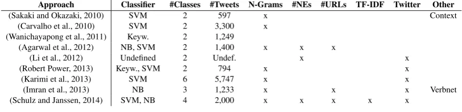
A review of existing work on the classification of social media content shows which features, feature groups and algorithms are generally used (see table 1). Furthermore, the number of classes and the dominating approaches unfold. We re-port the ratios of labeled tweets for the individual approaches; however, we omit performance mea-sures as these are directly related to the respective datasets used for evaluation.

Classifiers based on Support Vector Machines (SVM) or Naive Bayes (NB) clearly dominate in terms of performance for incident type

classifi-cation. (Sakaki and Okazaki, 2010; Carvalho et al., 2010; Agarwal et al., 2012; Robert Power, 2013; Schulz and Janssen, 2014) trained an SVM, whereas (Agarwal et al., 2012; Imran et al., 2013; Schulz and Janssen, 2014) also eval-uated an NB classifier. In contrast to these works, (Wanichayapong et al., 2011) followed a dictionary-based approach using traffic-related keywords. (Li et al., 2012) do not provide any in-formation about the classifier used.

Feature groups are mostly based on word-n-grams, such as unigrams (Carvalho et al., 2010), bigrams (Imran et al., 2013), or the combination of unigrams and bigrams (Robert Power, 2013; Karimi et al., 2013; Agarwal et al., 2012). (Schulz and Janssen, 2014) combined unigrams, bigrams, and trigrams. Also, based on the words present in the text named entities such as locations, organi-zations, or persons were used by (Agarwal et al., 2012; Li et al., 2012; Schulz and Janssen, 2014).

Twitter-specific features were also used, includ-ing the number of hashtags, @-mentions or web-text features such as the presence of numbers or URLs (Li et al., 2012; Agarwal et al., 2012; Robert Power, 2013; Karimi et al., 2013; Imran et al., 2013; Schulz and Janssen, 2014).

Keywords also play a crucial role in fea-ture design. (Sakaki and Okazaki, 2010) used earthquake-specific keywords, statistical features (the number of words in a tweet and the position of keywords), and word context features (the words before and after the earthquake-related keyword). (Wanichayapong et al., 2011) used traffic-related keywords in combination with location-related keywords. Furthermore, Li et al. (2012) itera-tively refined a keyword-based search for retriev-ing a higher number of incident-related tweets.

Two approaches rely on more specific feature groups. The approach of (Schulz and Janssen, 2014) is the only one that uses TF-IDF scores. (Imran et al., 2013) use Kipper et al.’s (2006) ex-tension of the Verbnet ontology for verbs.

The related approaches mostly use word-n-grams and a variety of Twitter-specific features. Datasets are spatially and temporally restricted and limited to a small number, complicating gen-eralizability.

3 Data Collection and Processing

Table 1: Overview of related approaches for incident type classification. (NEs = Named Entities)

Approach Classifier #Classes #Tweets N-Grams #NEs #URLs TF-IDF Twitter Other

(Sakaki and Okazaki, 2010) SVM 2 597 x Context

(Carvalho et al., 2010) SVM 2 3,300 x (Wanichayapong et al., 2011) Keyw. 2 1,249

(Agarwal et al., 2012) NB, SVM 2 1,400 x x x

(Li et al., 2012) Undefined 2 Undef. x x

(Robert Power, 2013) Keyw., SVM 2 794 x x

(Karimi et al., 2013) SVM 6 5,747 x x

(Imran et al., 2013) NB 3 1,233 x x x Verbnet

(Schulz and Janssen, 2014) SVM, NB 4 2,000 x x x x x

created in. For this purpose, we created 10 datasets with more than 20k labeled tweets to train and test models with respect to their generalization. In the following, we describe how this data was collected, preprocessed, and which features were generated.

3.1 Data Collection

We focus on tweets as suitable example for un-structured textual information shared in social me-dia. The classification of incident-related tweets represents a challenge that is relevant for many cities. We use a complex four-class classification problem, where new tweets can be assigned to the classes “crash”, “fire”, “shooting”, and a neutral class “not incident related”. This goes beyond re-lated work with a focus on two-class classification. Our classes were identified as the most common incident types in Seattle using the Fire Calls data set (http://seattle.data.gov), an official incident in-formation source.

As ground truth data, we collected several city-specific datasets using the Twitter Search API. These datasets were collected in a 15 km ra-dius around the city centres of Boston (USA), Brisbane (AUS), Chicago (USA), Dublin (IRE), London (UK), Memphis (USA), New York City (USA), San Francisco (USA), Seattle (USA), Syd-ney (AUS).

We selected these cities because of their huge regional distance, which allows us to evaluate our approaches with respect not only to geographi-cal, but also to cultural variations. Also, for all cities, sufficiently many English tweets can be re-trieved. We chose 15 km as radius to collect a rep-resentative data sample even from cities with large metropolitan areas. Despite the limitations of the Twitter Search API with respect to the number of geotagged tweets, we assume that our sample is, although by definition incomplete, highly relevant

to our experiments.

We collected all available Tweets during lim-ited time periods, resulting in three initial sets of tweets: 7.5M tweets collected from November, 2012 to February, 2013 for Memphis and Seattle (SET CITY 1); 2.5M tweets collected from Jan-uary, 2014 to March, 2014 for New York City, Chicago, and San Francisco (SET CITY 2); 5M tweets collected from July, 2014 to August, 2014 for Boston, Brisbane, Dublin, London, and Syd-ney (SET CITY 3).

For the manual labeling process, we had to se-lect a subset of our original tweet set which in-cluded our classes of interest for model training and testing. Generating subsets is required be-cause manual labeling of social media data is very expensive, especially if multiple annotators are involved. To generate subsets we used the ap-proach of (Schulz et al., 2013) of extracting mi-croposts using incident-related keywords. As a result, more than 200 keywords were identified for each class. Based on these incident-related keywords, we were able to accurately and effi-ciently filter the datasets. After applying keyword-filtering, we randomly selected 5.000 microposts for each city. Though one might assume that this pre-filtering leads to a biased dataset, (Schulz and Janssen, 2014) showed that keyword sampling does not influence the classification process as the performance of a keyword-based classifier is no-tably worse compared to supervised classifiers.

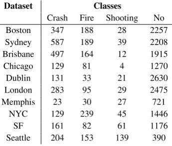
Table 2: Class distributions for all datasets.

Dataset Classes

Crash Fire Shooting No

Boston 347 188 28 2257

Sydney 587 189 39 2208

Brisbane 497 164 12 1915

Chicago 129 81 4 1270

Dublin 131 33 21 2630

London 283 95 29 2475

Memphis 23 30 27 721

NYC 129 239 45 1446

SF 161 82 61 1176

Seattle 204 153 139 390

which all coders agreed to at least 75%. In the case of disagreement, the tweets were removed. This resulted in ten datasets with regional diversity to be used for evaluation.

Table 2 lists the class distributions for each dataset. The distributions vary considerably, al-lowing us to evaluate with typical city-specific samples. Also, the “crash” class seems to be the most prominent incident type, whereas “shoot-ings” are less frequent. One reason for this is that “shootings” do not occur as frequent as other inci-dents, whereas another less obvious reason might be that people tend to report more about specific incident types and that there is not necessarily a correlation between the real-world incidents and those mentioned in tweets. Although the data sets have been filtered based on keywords, the “no in-cident” class remains the largest class.

One of the key questions that motivates our work is to which extent the used words vary in each dataset as an effect of the spatial and cultural context. We thus analysed how similar all datasets are by calculating the intersection of tokens. We found that after preprocessing, between 14% and 23% tokens are shared between the datasets. We do not assume that every unique token is a city-specific token, but the large number of tweets in our evaluations gives a first indication that there is a diversity in the samples that either requires the training of several individual- or one generalizing model which is the focus of this paper.

3.2 Preprocessing and Feature Generation To use our datasets for feature generation, i.e., for deriving differentfeature groupsthat are used for training a classification model, we had to convert the texts into a structured representation by means of preprocessing. Following this, we extracted

several features for training classification mod-els. To evaluate the best feature groups for inci-dent type classification, we re-implemented com-monly used feature extraction approaches from the state of the art. We further extended these feature groups by additional ones that seemed promising in this problem domain:

Preprocessing As a first step, the text was con-verted to Unicode to preserve non-Unicode char-acters. Specific URLs would not be useful for the classification process, therefore we replaced them with a common token “URL”. We then removed stopwords and conducted tokenization. Every token was then analysed and non-alphanumeric characters were removed or replaced. Finally, we applied lemmatization to normalize all tokens. All preprocessing steps were performed by DKPro TC (de Castilho and Gurevych, 2014), a popular framework for text classification. After prepro-cessing, we generated several features (see Table 3). In the following, we give a description of the different feature groups.

Baseline Feature Sets As the most simple ap-proach and as used in all related works, we repre-sented tweets as a set of words and also as a set of characters with varying lengths. As features, we used a vector with the frequency of each n-gram. Most importantly, we evaluated the powerset of all different combinations of n-grams. For instance, if a length ofn= 2was chosen, we evaluated the three combinations(n = 1),(n= 1,2),(n= 2). Furthermore, as not all tokens are necessarily im-portant for the classification process, we evaluated several top-k selection strategies, i.e., taking only thekmost frequent n-grams into account. For this, we testedk = 100,1000,5000as well as the ap-proach using all n-grams. We treat these features as the baseline approach, and extend it by addi-tional features, e.g. similarity, sentiment scores, Twitter-specific features.

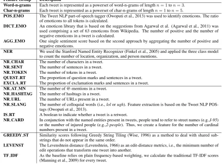
Table 3: Overview of all feature groups implemented for comparison

Feature Group Description

Word-n-grams Each tweet is represented as a powerset of word-n-grams of lengthn= 1ton= 3.

Char-n-grams Each tweet is represented as a powerset of char-n-grams of lengthn= 1ton= 5.

POS EMO The Tweet NLP part-of-speech tagger (Owoputi et al., 2013) was used to identify emoticons. The ratio of emoticons to all tokens is calculated.

DICT EMO An emoticon library that is based on the suggestions from Agarwal et al. (Agarwal et al., 2011) was used comprising a set of 63 emoticons from Wikipedia. The number of positive and the number of negative emoticons in a tweet is calculated.

AGG EMO One single sentiment score based on the second approach by aggregating the number of positive and negative emoticons.

NER We used the Stanford Named Entity Recognizer (Finkel et al., 2005) and applied the three class model to count the number of location, organization, and person mentions.

NR CHAR The number of characters in a tweet.

NR SENT The number of sentences in a tweet.

NR TOKEN The number of tokens in a tweet.

QUEST RT The proportion of question marks and sentences in a tweet.

EXCLA RT The proportion of exclamation marks and sentences in a tweet.

NR AT MN The number of @-mentions in a tweet.

NR HASHTAG The number of hashtags in a tweet.

NR URL The number of URLs present in a tweet.

NR SLANG The number of colloquial words (i.e.,lolorugh). Feature extraction is based on the Tweet NLP POS-tags (Owoputi et al., 2013).

IS RT A boolean to indicate whether a tweet is a retweet.

NR CARD In conjunction with the named entities present in tweets, people tend to refer to street names (e.g.,I-95) or the number of injured people (e.g.,2-people). Thus, we create a feature for the number of cardinal numbers present in a tweet.

GREEDY ST Similarity scores following Greedy String Tiling (Wise, 1996) as a method to deal with shared sub-strings that do not appear in the same order.

LEVENST The Levenshtein distance (Levenshtein, 1966) as an edit-distance metrics, i.e., the minimum number of edit operations that transform one tweet into another.

TF IDF As the baseline relies on plain frequency-based weighting, we calculate the traditional TF-IDF scores (Manning et al., 2009) for every tweet.

Named Entities: As shown in the state of the art, named entities, i.e. entities that have been assigned a name such as Seattle, are commonly used in tweets. Named entities might be valuable, as these are used frequently in incident-related tweets. Thus, we also incorporated Named Entity Recognition (NER) for feature extraction.

Stylistic Features: The style of a tweet could be an additional indicator for incident relatedness. For instance, a repetition of punctuations could point at a person that is expressing emotions re-sulting from an ongoing incident. Structured rep-resentation might indicate high quality.

Twitter-specific features As shown in related work, several Twitter-specific features seem to be valuable for incident type classification such as the number of @-mentions and hashtags.

Similarity Features The similarity of individual tweets might be helpful to identify common top-ics. We therefore implemented several similarity

scores1_{. The rationale behind this is to embrace}

additional features that do not only take the raw frequencies of words into account, but also which words appear in which document.

To sum up, we re-implemented two approaches that will serve as a baseline, and 18 additional fea-ture groups to extend them. In the following sec-tion, we will evaluate the usefulness of these ap-proaches for training a generalizing model.

4 Evaluation

4.1 Method

The indicators for well-performing features in re-lated work allows us to perform a condensed evaluation, compared to similar studies such as (Hasanain et al., 2014).

Our approach comprises three steps: First, we evaluated the baseline approaches, i.e., word- and char-n-grams. Second, we combined each of the remaining features with the best performing base-line feature. Third, we again selected the best per-forming combinations and evaluated their power set. To evaluate the suitability of different features for training generalizing models, we picked one dataset from the 10 presented in Section 3.1 for training, and tested on the remaining 9 datasets. We did not evaluate different models on datasets from only one city, as we were interested in gen-eralizing models.

Selecting each city as training set resulted in 90 performance samples per model. The models were formed by combining the feature sets described in the previous section 3.2 or respectively, their com-binations, with an SVM and NB classifier. We de-cided for these classification algorithms since they were the most successful in related work. Another reason for the choice of NB is its good perfor-mance in text classification tasks, as demonstrated by Rennie et al. (2003). We relied on the Lib-Linear implementation of an SVM because it has been shown that for a large number of features and a small number of instances, a linear kernel is comparable to a non-linear one (Hsu et al., 2003). As for SVMs parameter tuning is inevitable, we evaluated the best settings for the slack variable c whenever an SVM was used. For training and testing, we used the reference implementations in WEKA (Hall et al., 2009).

We calculated the F1-Measure for assessing performance, because it is well established in text classification, cannot be manipulated by the classi-fication threshold parameter and allows to measure 1_{The respective similarity scores have been calculated on}

the whole document corpus after preprocessing.

the overall performance of the approaches with an emphasis on the individual classes (Jakowicz and Shah, 2011). In Section 3.1, we demonstrated that the proportion of data representing individ-ual classes varies strongly. We therefore weighted the F1-measure by this ratio and report the micro-averaged results over all datasets F1. Given our focus on training a generalizable model, we delib-erately did not focus on the performance variation in the individual datasets.

4.2 Results

In order to check whether our findings persist at least across the two learning algorithms, we did not aggregate the model performance samples but analyzed them for each algorithm separately. We therefore only have one independent variable, our feature groups, that affects the model perfor-mance. In order to keep p-value inflation low, we only compared the ten best performing models for each algorithm with respect to the F1-Measure. Note that even if the difference in performance be-tween these models appears small, there are thus many worse models that were not explicitly listed. Our samples generally do not fulfill the assump-tions of normality and sphericity required by para-metric tests for comparing more than two groups. Under the violation of these assumptions, non-parametric tests have more power and are less prone to outliers (Demsar, 2006). We therefore relied exclusively on the non-parametric tests sug-gested in literature: Friedman’s test was used as non-parametric alternative to a repeated-measures one-way ANOVA, and Nemenyi’s test2 _{was used}

post-hoc as a replacement for Tukey’s test. In contrast to its parametric counterpart, Fried-man’s test is based on a ranking of the models in-duced by the performance measure, and therefore only relies implicitly on the latter. Each model is ranked from best to worst, with mean ranks being 2_{We chose Nemenyi’s test because it is widely accepted}

in the machine learning community. A discussion of alterna-tives can be found in Herrera et al. (Herrera, 2008).

Feature Group words(1000,1,2) words(1000,1,3) words(ALL,1,1) words(5000,1,1) words(100,1,1) words(100,1,2) words(100,1,3) words(5000,1,3) words(1000,1,1) words(5000,1,1)

F1 82.10 82.00 82.86 82.87 80.62 80.66 80.76 81.15 82.71 81.28

(a) LibLinear

Feature Group words(1000,1,2) words(1000,1,3) words(1000,1,1) words(5000,1,2) chars(5000,2,3) chars(5000,2,4) chars(1000,2,4) chars(1000,2,5) chars(1000,2,3) chars(5000,2,5)

F1 80.10 79.56 80.10 78.09 78.01 80.27 80.22 79.73 79.86 80.48

(b) NaiveBayes

used in case of ties. TheFriedman statisticis cal-culated by dividing the sum of squares of the mean ranks by the sum of squares error. For sufficiently many samples, the statistic follows aχ2

distribu-tion withk−1degrees of freedom. Theq statistic

used in Nemenyi’s test is similar to the one used by Tukey, but uses rank differences. It utilises the previous ranking from the Frieman test to calcu-late and recalcu-late the average ranks of two models, for each available pair. Two models are consid-ered significantly different, if their difference in mean ranks exceeds a critical value, which varies for different significance levels. For a detailed de-scription and examples of these tests, see (Jakow-icz and Shah, 2011).

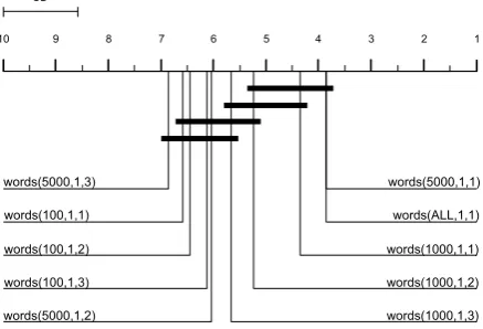
We illustrated the ranks and significant differ-ences between the feature groups by means of the critical difference (CD) diagram. Introduced by Demsar (2006), this diagram lists the feature groups ordered by their rank, where lower rank numbers indicate higher performance. Feature groups are connected with bars if they are not sig-nificantly different, givenα= 0.05.

In the following, we will use shortcuts like

words(1000,1,2)to denote the 1000 most frequent

uni- and bigrams. The same applies for char-n-grams. Abbreviations can be found in Table 3. 4.2.1 Evaluation using LibLinear Classifier We first evaluated which of our 20 baseline fea-ture sets, as described in Section 3, lead to the best classification performance over different datasets. Notably, the ten best-performing approaches were all combinations of word-n-grams. Table 4 contains the average F-Measures for these ap-proaches. The Friedman test indicated strong sig-nificant differences between the performances of these groups (χ2

r(9) = 112.467, p < 0.001, α =

0.01). The subsequent Nemenyi test indicated strong significant pairwise differences between the performances of the models (α = 0.01), with p-values listed in Table 2 in the supplementary.

Figure 1 illustrates the differences by means of a CD diagram: the approaches of using simple un-igrams of the most frequent 5000 and all words provide the best results, i.e. they have the lowest rank. They are not significantly different from the 1000 most frequent word-uni and bigrams. Never-theless, they are significantly better than all other baseline approaches.

This also applies to the char-n-gram ap-proaches, that were not considered in this

statisti-CD

10 9 8 7 6 5 4 3 2 1

words(5000,1,1)

words(ALL,1,1)

words(1000,1,1)

words(1000,1,2)

words(1000,1,3) words(5000,1,2)

words(100,1,3) words(100,1,2) words(100,1,1) words(5000,1,3)

Figure 1: CD diagram with the ranks of the ten best performing baseline feature groups for Lib-Linear. Feature groups are connected if they are not significantly different (α= 0.05).

cal comparison due to their inferior performance. It is important to note that the differences between the worst word-n-gram approaches and the best char-n-gram approaches could still be statistically non-significant.

The best performing baseline approach for LibLinear is using unigrams of the top 5000 words, i.e. words(5000,1,1), with F1 = 82.87. We therefore picked this baseline feature group for the second part of our evaluation. We added each non-baseline feature individually to the selected baseline approach and compared the performances of these combinations and the non-extended base-line group. Table 6 lists the averaged F-Measure. When comparing the ten best-performing groups, the Friedman test showed strong significant dif-ferences between the performances of the models (χ2

r(9) = 87.274, p < 0.001, α = 0.01). The

Nemenyi test partly showed strong significant dif-ferences between the performances of the models (for the corresponding p-values see Table 3 in the supplementary). They are illustrated in the CD di-agram in Figure 2. The tests indicate that adding

NERandNR AT MTto the baseline approach

pro-vides the best performances withF1 = 83.32and F1 = 83.03respectively.

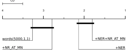
Finally, we evaluated the power set of these feature groups, i.e. we compared the individual groups and their combination. Table 5 contains the corresponding averaged F-Measures. For the resulting performance samples, the Friedman test showed strong significant differences between the models (χ2

r(3) = 72.014, p < 0.001, α = 0.01).

CD

10 9 8 7 6 5 4 3 2 1

NER

NR_AT_MN

NR_CARD

QUEST_RT

EXCLA_RT IS_RT

DICT_EMO 5000,1,1 NR_SLANG POS_EMO

words( )

Figure 2: CD diagram with the ranks of the ten best performing feature groups for LibLinear, comprising the baseline and the baseline with an additional feature. Feature groups are connected if they are not significantly different (α= 0.05).

Feature Group words(5000,1,1) +NER +NER+NR AT MN +NR AT MN

F1 82.87 83.32 83.48 83.03

Table 5: Average F1-MeasureF1for the power set of best performing feature groups and LibLinear.

differences (α = 0.001), with p-values listed in Table 4 in the supplementary and illustrated in Fig-ure 3. The diagram shows that the combination

ofNERandNR AT MNwith thewords(5000,1,1)

baseline outperforms all other models with respect to F1 (F1 = 83.48), but does not differ sig-nificantly from the plain NER approach (F1 = 83.32). This combination gives us the final and best feature set for training a generalizing model over our datasets. As can be seen, the plain n-gram approach (F1 = 82.87) can be improved further by0.5%.

4.2.2 Evaluation using Naive Bayes Classifier In this section, we repeat the previous steps for the NB classifier. As baseline feature sets, we first evaluated the word-n-gram and char-n-gram ap-proaches. The averaged F-Measures can be found in Table 4. The Friedman test showed strong sig-nificant differences between the performances of the models (χ2

r(9) = 110.293, p < 0.001, α =

0.01). The Nemenyi test partly showed strong sig-nificant differences between the performances of the models (for the corresponding p-values see Ta-ble 1 in the supplementary). In contrast to the Li-bLinear classifier, using the 5000 most frequent combinations of two to five subsequent charac-ters, i.e.chars(5000,2,5)provide the best F1 score (F1 = 80.48). Thus, char-n-grams outperform the

CD

4 3 2 1

words(5000,1,1)

+NR_AT_MN

+NER+NR_AT_MN

+NER

Figure 3: CD diagram with the ranks of the best baseline feature groups, complemented with a combination of the best performing feature sets, for LibLinear. Feature groups are connected if they are not significantly different (α = 0.05).

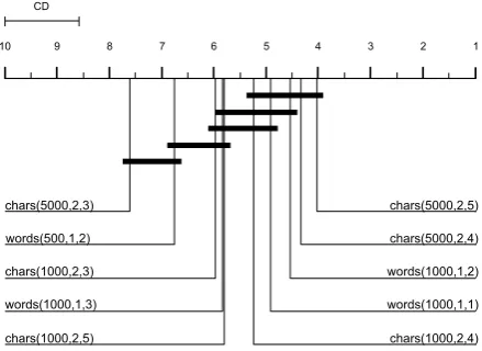
word-n-gram approaches with respect to F1. The CD diagram in Figure 5 shows that using either the 5000 most frequent char-n-grams with a length of two to five and two to four respec-tively, the 1000 most frequent word-n-grams with a length of one and one to two respectively, and the 1000 most frequent char-n-grams with a length of two to four do not differ significantly. However, using either the 5000 most frequent char-n-grams with a length of two to five and two to four respec-tively significantly outperform all other baseline approaches. As a subsequent step, we added each single feature tochars(5000,2,5)as the best base-line approach to find if these provide better per-formance for the NB classifier. Table 6 contains the corresponding averaged F-Measures. Though the Friedman test indicated strong significant dif-ferences between the performances of the mod-els (χ2

r(9) = 22.209, p = 0.008, α = 0.01), the

subsequent Nemenyi test did not indicate signifi-cant pairwise differences. We can therefore not re-peat the third step of our evaluation, but infer that for a NB classifier, the plain char-n-gram-based approach is sufficient for training a generalizing model for our dataset.

The results indicate that LibLinear provides a better avg. performance (F1 = 83.32) when train-ing a generaliztrain-ing model, compared to the NB classifier (F1 = 80.48).

5 Conclusion and Future Work

Feature Group words(5000,1,1) +DICT EMO +NER +NR CARD +NR AT MN +POS EMO +NR SLANG +EXCLA RT +QUEST RT +IS RT

F1 82.87 82.87 83.32 83.06 83.03 82.87 82.87 82.88 82.88 82.88

(a) LibLinear

Feature Group chars(5000,2,5) +DICT EMO +QUEST RT +NER +NR AT MN +NR HASHTAG +POS EMO +NR SLANG +NR SENT +EXCLA RT

F1 80.48 80.48 80.49 80.55 80.51 80.48 80.48 80.48 80.48 80.50

(b) NaiveBayes

Table 6: Average F1-MeasureF1for the ten best performing combinations of the best baseline and an additional feature

CD

10 9 8 7 6 5 4 3 2 1

chars(5000,2,5)

chars(5000,2,4)

words(1000,1,2)

words(1000,1,1)

chars(1000,2,4) chars(1000,2,5)

words(1000,1,3) chars(1000,2,3) words(500,1,2) chars(5000,2,3)

Figure 4: CD diagram with the ranks of the ten best performing baseline feature groups for Naive Bayes. Feature groups are connected if they are not significantly different (α = 0.05).

Figure 5: Ranks of NB baseline feature groups.

for the LibLinear and NB classification algorithms on ten spatially and temporally diverse datasets. The resulting F1-measure samples indicate that training a generalizing model, i.e., a model that is applicable on previously unseen incident-related data, is still a challenging task. We found that Li-bLinear provides a better averaged performance compared to the NB classifier. More surpris-ingly, additional feature groups that are commonly used in related work do not necessarily outperform a plain n-gram-based approach. This highlights the need for other novel approaches for training generalizing classification models. Especially in the domain of incident detection and emergency management, our findings are important because less time consuming techniques showed nearly the same performance as sophisticated ones.

There are two main topics for our future work. First, we will investigate the performance of mod-els generated with biased datasets on unfiltered datasets. This is relevant, if a technique like filter-ing is used to include more relevant class examples

in a dataset than provided with an original sample – a necessary step to realize a labeled dataset for model learning of a rare-class task. Second, we will work on using novel features for the creation of generalized models. One example is the uti-lization of the Semantic Web to generate abstract features, utilizing a technique called Semantic straction (Schulz et al., 2015a). Semantic Ab-straction has shown to improve the generalization of tweet classification by deriving features from Linked Open Data and using location and tempo-ral mentions.

References

Apoorv Agarwal, Boyi Xie, Ilia Vovsha, Owen Ram-bow, and Rebecca Passonneau. 2011. Sentiment analysis of twitter data. InProceedings of the Work-shop on Languages in Social Media, LSM ’11, pages 30–38. ACL.

Puneet Agarwal, Rajgopal Vaithiyanathan, Saurabh Sharma, and Gautam Shroff. 2012. Catching the long-tail: Extracting local news events from twitter. InProceedings of the Sixth International Conference on Weblogs and Social Media, ICWSM 2012. AAAI Press.

S. Carvalho, L. Sarmento, and R. J. F. Rossetti. 2010. Real-time sensing of traffic information in twitter messages. In Proceedings of the 4th Workshop on Artificial Transportation Systems and Simulation ATSS, ITSC’10, pages 19–22. IEEE Computer Soci-ety.

Richard Eckart de Castilho and Iryna Gurevych. 2014. A broad-coverage collection of portable nlp compo-nents for building shareable analysis pipelines. In

Proceedings OIAF4HLT at COLING 2014, pages 1– 11.

Janez Demsar. 2006. Statistical Comparisons of Clas-sifiers over Multiple Data Sets. Journal of Machine Learning Research, 7:1–30.

Alec Go, Richa Bhayani, and Lei Huang. 2009. Twit-ter sentiment classification using distant supervision. InProceedings of the Workshop on Languages in So-cial Media, LSM ’11, pages 30–38. Association for Computational Linguistics.

Mark Hall, Eibe Frank, Geoffrey Holmes, Bernhard Pfahringer, Peter Reutemann, and Ian H. Witten. 2009. The weka data mining software: an update.

SIGKDD Explor. Newsl., 11(1):10–18.

Maram Hasanain, Tamer Elsayed, and Walid Magdy. 2014. Identification of answer-seeking questions in arabic microblogs. InProceedings of the 23rd ACM International Conference on Conference on Infor-mation and Knowledge Management, pages 1839– 1842. ACM.

Francisco Herrera. 2008. An Extension on Statistical Comparisons of Classifiers over Multiple Data Sets for all Pairwise Comparisons. Journal of Machine Learning Research, 9:2677–2694.

Chih-Wei Hsu, Chih-Chung Chang, and Chih-Jen Lin. 2003. A practical guide to support vector classifi-cation. Technical report, Department of Computer Science, National Taiwan University.

Muhammad Imran, Shady Elbassuoni, Carlos Castillo, Fernando Diaz, and Patrick Meier, 2013. Extract-ing information nuggets from disaster- Related mes-sages in social media, pages 791–801. Karlsruher Institut fur Technologie (KIT).

Nathalie Jakowicz and Mohak Shah. 2011. Evaluating Learning Algorithms. A Classification Perspective. Cambridge University Press, Cambridge.

Sarvnaz Karimi, Jie Yin, and Cecile Paris. 2013. Clas-sifying microblogs for disasters. InProceedings of the 18th Australasian Document Computing Sympo-sium, ADCS ’13, pages 26–33. ACM.

Karen Kipper, Anna Korhonen, Neville Ryant, and Martha Palmer. 2006. Extending verbnet with novel verb classes. InProceedings LREC’06.

VI Levenshtein. 1966. Binary Codes Capable of Cor-recting Deletions, Insertions and Reversals. Soviet Physics Doklady, 10:707.

Rui Li, Kin Hou Lei, Ravi Khadiwala, and Kevin Chen-Chuan Chang. 2012. Tedas: A twitter-based event detection and analysis system. InProceedings of the 28th International Conference on Data Engineering, ICDE’12, pages 1273–1276. IEEE Computer Soci-ety.

Christopher D. Manning, Prabhakar Raghavan, and Hinrich Schtze., 2009. An Introduction to Informa-tion Retrieval, pages 117–120. Cambridge Univer-sity Press.

Olutobi Owoputi, Chris Dyer, Kevin Gimpel, Nathan Schneider, and Noah A. Smith. 2013. Improved part-of-speech tagging for online conversational text with word clusters. InIn Proceedings of NAACL. Jason D. Rennie, Lawrence Shih, Jaime Teevan, and

David R. Karger. 2003. Tackling the poor assump-tions of naive bayes text classifiers. In Tom Fawcett and Nina Mishra, editors,International Conference on Machine Learning (ICML-03), pages 616–623. AAAI Press.

David Ratcliffe Robert Power, Bella Robinson. 2013. Finding fires with twitter. In Australasian Lan-guage Technology Association Workshop, pages 80– 89. Association for Computational Linguistics.

Takeshi Sakaki and M Okazaki. 2010. Earthquake shakes twitter users: real-time event detection by social sensors. InProceedings of the 19th interna-tional conference on World Wide Web, WWW ’10, pages 851–860. ACM.

Axel Schulz and Frederik Janssen. 2014. What is good for one city may not be good for another one: Eval-uating generalization for tweet classification based on semantic abstraction. In CEUR, editor, Proceed-ings of the Fifth Workshop on Semantics for Smarter Cities a Workshop at the 13th International Seman-tic Web Conference, volume 1280, pages 53–67.

Axel Schulz, Petar Ristoski, and Heiko Paulheim. 2013. I see a car crash: Real-time detection of small scale incidents in microblogs. InESWC’13, pages 22–33.

Axel Schulz, Christian Guckelsberger, and Frederik Janssen. 2015a. Semantic abstraction for gener-alization of tweet classification: An evaluation on incident-related tweets. In Semantic Web Journal: Special Issue on Smart Cities.

Axel Schulz, Benedikt Schmidt, and Thorsten Strufe. 2015b. Small-scale incident detection based on mi-croposts. InProceedings of the 26th ACM Confer-ence on Hypertext and Social Media. ACM.

N. Wanichayapong, W. Pruthipunyaskul, W. Pattara-Atikom, and P. Chaovalit. 2011. Social-based traf-fic information extraction and classitraf-fication. In Pro-ceedings of the 11th International Conference on ITS Telecommunications, ITST’11, pages 107–112. IEEE Computer Society.

Michael J. Wise. 1996. Yap3: Improved detection of similarities in computer program and other texts. In