Online Full Text

(1)

Abstract — This research aims to study and improve processes and production lines of erbium doped fibre amplifiers using lean manufacturing systems via an application of computer simulation. It is currently complicated for this process to meet the customers’ requirement under a present economic climate that products need to be shipped to customers as soon as possible after purchases ordered. The concepts of lean manufacturing are applied through a computer simulation with three scenarios of lean tooled box systems. Firstly, the production schedule based on shipment date is combined with a first in first out control system. The second scenario focuses on a designed flow process plant layout. Finally, the previous flow process plant layout combined with production schedule based on shipment date including the first in first out control systems. The most preferable scenario from a computer simulation is selected to implement to the real production process of erbium doped fibre amplifiers. A comparison is carried out to determine the actual performance measures via an analysis of variance of the production time per unit achieved via each scenario. The goodness of an adequacy of the linear statistical model via experimental errors or residuals is also performed to check the normality, constant variance and independence of the residuals. The results show that a hybrid scenario of lean manufacturing system with the first in first out control and flow process plant lay out leads to better performance in terms of the mean and variance of production times.

Index Terms — Erbium Doped Fibre Amplifier, Lean

Manufacturing, Computer Simulation, Flow Process Plant Layout, Analysis of Variance.

I. INTRODUCTION

The excellent optical amplifiers are available in forms of erbium doped fibre amplifiers (EDFA) and their uses were firstly reported in 1987 [1]. Currently, EDFA are the most widely used and therefore these are taken as standard amplifiers in all optical communication systems. They can

Manuscript received December 29, 2009. This work was supported in part the Thailand Research Fund (TRF), the National Research Council of Thailand (NRCT) and the Commission on Higher Education of Thailand. The authors wish to thank the Faculty of Engineering, Thammasat University, THAILAND for the financial support.

*T. Maneechote is with the Industrial Statistics and Operational Research Unit (ISO-RU), Department of Industrial Engineering, Faculty of Engineering, Thammasat University, 12120, THAILAND, [Phone: 662-564-3002-9; Fax: 662-564-3017; e-mail: [email protected], [email protected]]

P. Luangpaiboon is an Associate Professor, ISO-RU, Department of

Industrial Engineering, Faculty of Engineering, Thammasat University, 12120, THAILAND.

serve both as booster amplifier in the transmitter and as preamplifier in the receiver [2]. EDFA offers several advantages when compared. They are commercially available in both C (the original frequency allocation used for communication satellites) and L (the frequency long range between 390MHz and 1.55GHz used for communication satellites) and offer high gain with relatively low noise figure. However, EDFA adds some complexities, such as a pump laser, to a system. Integration with other components is also required as shown in Fig. 1. For a schematic process of EDFA focusing on many components need to be integrated with fibre optic, these make a module assembly process is complicated.

Today various industries are highly competitive due to the increasing market demand as well as the current economic climates make impact to every industry around the world, especially electronics. Several manufacturers then need to have improvements in quality, production costs, lead time reduction for shipment and contract manufacturer consideration. Aims are to reduce the economic risk and eliminate fixed cost to handle. The area of this research is merely focusing on contract manufacturing for erbium doped fibre amplifier. The process should practically produce erbium doped fibre amplifiers to deliver to customers [3]. However, the behaviour of current manufacturing process is to integrate all batches and sizes, this turns to be currently one of the most important problems for the optical communication system company.

Fiber

EDF Amplified signal out

Isolator Fiber Coupler

Weak signal in Isolator Fiber

Pump

Fig.1 Schematic Process of Erbium Doped Fibre Amplifier. There are also various types of industrial wastes in production processes. Waste which impacts the production time is over due for a planned shipment. The current manufacturing conditions of the EDFA process provide incapable production time to meet customers’ requirement including high variation and this leads to a process improvement (Fig. 2). There are some real risks of having a part borderline out of specification for this process as considered via the loss function of Taguchi.

Lean manufacturing is one of improvement ways that are considered to eliminate waste and improve the production lead time to produce finished goods. Seven types of industrial

Production Time Reduction for

Erbium Doped Fibre Amplifier Process via

Lean Manufacturing Systems

(2)

wastes that the lean strategy tries to eliminate from the production frame consist of:

1. Overproduction or manufacturing products more than customers need;

2. Inventory or any supply in excess amounts of required products;

3. Waiting or idle operator or machine time;

4. Motion or movement of people or machines which does not provide value added;

5. Transportation or any material movement that does not directly support value added operations;

6. Defects or making defective parts; and

7. Extra processing or any processes that do not lead to value added to products [4].

36 30 24 18 12 6 0

LSLTargetUSL

LSL 2

Target 5

U SL 9

Sample M ean 12.8316

Sample N 944

StDev (Within) 5.881

StDev (O v erall) 6.5661 P rocess Data

C p 0.20

C P L 0.61

C P U -0.22

C pk -0.22

P p 0.18

P P L 0.55

P P U -0.19

P pk -0.19

C pm 0.10

O v erall C apability P otential (Within) C apability

P P M < LSL 1059.32

P P M > U SL 537076.27

P P M Total 538135.59

O bserv ed P erformance

P P M < LS L 32752.83

P P M > U SL 742643.55

P P M Total 775396.38

Exp. Within P erformance

P P M < LSL 49510.43

P P M > U SL 720234.28

P P M Total 769744.72

E xp. O v erall P erformance

Within Ov erall

[image:2.595.47.290.255.394.2]

Process Capability of Production time

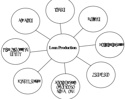
Fig.2 The Current Process Capability of the EDFA Process. Lean production organisations achieve some benefits by eliminating these types of waste or non-value creating activities using a set of tools and principles [5]. Eight tools that embrace the concept of lean manufacturing are successfully utilised in the current manufacturing process. These consist of Cellular Layouts, Single Minute Exchange of Die (SMED), Andon Boards, Jidoka, Heijunka, Six-sigma, Flow Process and Kanban Systems and Poka-Yoke as shown in Fig. 3. Using these concepts, it seems to aid in bridging the gap between the empirical and conceptual worlds.

Poka-Yoke Cellular layouts

Single munute exchange of die (SMED) Andon Boards

Flow process and Kanban

Six Sigma Heijunka

Jindoka

Lean Production

Fig. 3 Concept Map of Lean Production.

Cellular Layouts refer to the arrangement of assembly line operations into small U-shaped cells. Being spatial in nature,

cellular layouts are quite easy to use of illustrations, to show how much walking distance an assembler might have to in a typical shift and the cost saving to be derived from it.

Andon Boards are signal systems that are employed to notify operators about the status of the system (i.e. assembly line).

Jidoka or automation with a human touch is another concept that is very integral to lean production’s definition. By giving automated machinery, the ability to identify problem with their own work gives them the ability, not only to detect problems but also to correct them if they are capable of doing. Heijunka, this concept refers to the way in which jobs are scheduled. By keeping the production constant, variability that is due to sporadic customer demand does not force the assembly line to have work-in-process when demand is low and too little when demand is high. Little’s law of variability buffering is used to re-enforce this concept.

Six-Sigma is another manufacturing improvement strategy that has gained widespread usages.

Flow Process and Kanban Systems are lot or batch control techniques with the proper flow process design for line balancing to eliminate the waiting time and bottle neck.

Heijunka and Single Minute Exchange of Die or SMED are techniques in the maintenance of a constant work flow throughout the assembly line.

Poka-Yoke or mistake proofing systems are used to prevent both humans and machines from making mistakes [6].

Lean production concepts were analysed for all of tools to select the significant lean concept before performing a simulation. It will be combined with other improvement concepts which are considered to be high potential to improve the current problem in erbium doped fibre amplifier. From a benchmarking of experts, an analysis of the lean production selection is determined via score that are given to all lean tools based on three criteria (Table 1). They consist of possibility, frequency and risk. Firstly, the possibility is to identify how potential to implement any lean production tool into the erbium doped fibre amplifier manufacturing process. The most possibility will start from the highest of 4 to the lowest of 1 scores. Secondly, the frequency is to identify how frequent does the over lead time production happen if any lean production tool is not implemented into erbium doped fibre amplifier manufacturing process. The most frequency will start from 4 to 1 scores. Finally, the risk is to indentify how much the erbium doped amplifier manufacturing process does risk if there is no implementation of any lean production tools. The most risk will start from 4 to 1 scores. The total score for each lean’s tool was eventually determined from the multiplication of all criteria. The most important lean production tool was identified and selected to be the significant tool to a computer simulation in the next step by taking account of the highest levelled score.

[image:2.595.63.273.536.702.2]

(3)

[image:3.595.312.545.263.542.2]

the process implementation or improvement without interruption in a current production.

TABLE 1 Analysis of Lean Production Selection for Computer Simulation

Lean’s Tools Possibility Frequency Risk Total

Cellular

Layouts 1 2 1 2

Andon Boards 1 1 1 1

Jidoka 1 1 2 2

Six-Sigma 1 1 2 2

Flow Process and Kanban

System 3 2 2 12

Heijunka 1 1 1 1

SMED 1 1 1 1

Poka-Yoke 1 2 1 2

The objectives of this research are to analyse and create the current problem model with one-piece operation through a computer simulation, to compare with three creation simulation models with lean’s tool to improve the complex manufacturing process and to improve a manufacturing process to be a flow process with the reduced production time. In this research, the more preferable lean tool via an analysis of variance will be finally applied to the real process of EDFA. This paper is organised as follows. Section II describes the current manufacturing process of EDFA. Sections III and IV are briefing about related research methods and simulation results. Section V illustrates simulation implementations. The conclusion is also summarised in Section VI and it is followed by acknowledgment and references.

II. THE CURRENT MANUFACTURING PROCESS OF ERBIUM

DOPED FIBRE AMPLIFIER

In the case study of the erbium doped fibre amplifier product, there are various shapes and sizes of the products and they can be categorised in to two types of A and B. There are some differences between these types. Products categorised A have to down load both firmware and software while products categorised B need to down load only a firmware into the module and a pre test process.

Nowadays, production line consists of six procedures: (1) a kitting process to optimise the parameters of each component and successfully match all as a good module via a computer program, (2) a soldering process to install the optical components to the print circuit board, (3) an assembly process to assemble all optical, electrical and mechanical components into the module at the assembly station and contain a splicer to splice fibre in each component, (4) a pre test process to measure the passive components and pre communicate between the print circuit board and its components, (5) a final test process to perform a calibration for all active components in the module and to measure overall modules’ operations called as a functional test and (6) a final inspection process to attach all labels and packages including a visual inspection to ensure that all conditions are met to customers’ specification.

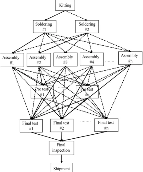
Optical fibre is a part of the product that its manufacturing process is different from generic products. It needs high skill of operators because the assembly is performed to connect all optical or fusion splicing components together. The process with the low loss and high strength welded joint is formed between two optical fibre components [7]. This brings high levels of all production time of the EDFA process. Manufacturing layout and processes need to be suitably designed to produce a one-piece production [8]. There is also an insufficiency production management with no hierarchy of production procedures that affects the high level of work in process (WIP) as shown in Fig. 4. In general, the current process flow design is not suitable to the erbium doped fibre amplifier production due to the waste involved in the production. This situation leads to excessive production times.

. . . .

. . .

Soldering #2 Soldering

#1

Assembly #1

Assembly #2

Assembly #3

Assembly #4

Assembly #n

Final test #2 Final test

#1 Pre test

#1

Kitting

Final inspection

Shipment

Pre test #n

Final test #n

Fig.4 Erbium Doped Fibre Amplifier Process Flow. III. RESEARCH METHODS

(4)

Computer simulation modelling refers to as a broad collection of methods and applications, which mimic on a computer to study the behaviour of some real world systems or hypothetical situations using appropriate software. It is used to also determine how the system works by changing variables. Computer simulation modelling is applicable to almost any types of systems with any degrees of complexity. It is also very useful in analysing the behaviour of dynamic systems when compared. The dynamic systems are evolving over time through a succession of stochastically driven critical events in which complex interactions can occur between system components. Simulation does not only enable the behaviour of complex systems to be better understood. In the context of a system design, it also has a predictive and an evaluative capability, which allows the dynamic alternative designs or specific features of designs to be compared before the system is actually built. During simulating the behaviour of existing systems, it is possible to experiment with the effects of making various types of change to the system, either in terms of the configuration or operating environment in advance of actually making the change to the real system itself. This would be prohibitively expensive, requires very long time-scales, and possible to be financially disastrous.

The ARENA software is used to construct three simulation models as followed [11]. The production rate, total time, WIP and waiting time schedule are key performance factors to decide which process layout is the most appropriate. The common conditions for the manufacturing process of EDFA are (1) two soldering stations, (2) seven assembly stations, (3) one pre tester station, (4) two final tester stations and (5) one final inspection station. In the simulation, there is only one production line to be considered.

Scenario L1 - the production schedule is based on the shipment date with the first in first out (FIFO) control system. It is different from the current system because there is no due date consideration. This model is similarly simulated as the current process situation, but it includes the assignment of due dates on the logistic-manufacturing network information. The manufacturing, transportation, and supplier elements are integrated into a simulation model of the system to help the assignment of reliable delivery dates [12].

. . . . .

Kitting

Soldering#2 Soldering#1

Assembly#1 Assembly#2

Pre test Final test#1

Final test#2 Final

Inspection Process(FIP) Delivery

[image:4.595.311.545.145.250.2]

Assembly#7

Fig. 5 Schematic Procedures for Scenario L1.

Scenario L2 –flow process is considered to determine its performance. This model is used to simulate the designed flow process of the current system that there is no due date or schedule or the first in first out control. The purpose of this

model is to minimise the operation time of each job in the operation assembly. In the minimal total production time, it is necessary to specific the order in each job of various machines and process steps [13].

. . . .

Kitting

Final test#2 Final

[image:4.595.311.547.408.529.2]

Assembly#7

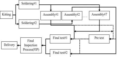
Scenario L3 – this includes the designed flow process, the production schedule based on shipment date and the FIFO control systems. This model is used to simulate the jobs that move through all processes to balance the operating time in each stage. The scheduling system is proposed and developed for a special type of the designed flow process. In this flow shop there is one assembly in each stage. Each job may require multiple operations in each stage [13]. The most effective model will be implemented into actual manufacturing lines to measure its performances.

. . . . Kitting

Final test#2 Final

Assembly#7

A comparison of experimental results of the most preferable from the simulation and the current manufacturing scenarios is made via a statistic tool called as an analysis of variance (ANOVA). In industrial processes, the design of experiments can be used to systematically investigate the process or product variables that influence product quality performances. Design of experiments allows collecting data at combinations of process or product variables, and then the significant findings are used to adjust manufacturing conditions. After the process conditions and product components, influencing product quality, are identified a direct sequential improvement efforts enhance a product's manufacturability, reliability, quality, and field performance.

[image:4.595.51.288.567.682.2]

(5)

experiment, varying the levels of the variables simultaneously rather than one at a time is efficient in terms of time and cost, and also allows for the study of interactions between the factors. Interactions are the driving force in many processes. Analysis of variance (ANOVA) is used to investigate and model the relationship between a response and one or more independent variables.

It is important to examine the goodness of an adequacy of the linear statistical model via experimental errors or residuals. Firstly, an exploratory tool called as a normal plot of residuals to show general characteristics of the data including typical values, spread or its variation, and shape, unusual values in the data tests to assess the normality of the residuals. Generally, the design points in this plot should form a straight line if the residuals are normally distributed. If the points on the plot depart from a straight line, the normality assumption may be invalid. If your data have fewer than 50 observed data, the plot may show curvature in the tails even if the residuals are normally distributed. With much easier, the Anderson-Darling statistic may be used to assess whether the residuals are normally distributed. If the P-Value is lower than the chosen significance level, the data do not follow a normal distribution. A plot of residuals versus fits should be used to show a random pattern of residuals. If a design point lies far from the majority of design points, it may be an outlier. Also, there should not be any recognisable patterns in this plot. A series of increasing or decreasing design points, a predominance of positive residuals, or a predominance of negative residuals patterns, such as increasing residuals with increasing fits may indicate experimental error that is not random. Residuals versus order is a plot of all residuals in the order that the data was collected and can be used to find non-random error, especially of time-related effects. A positive correlation is indicated by a clustering of residuals with the same sign. A negative correlation is indicated by rapid changes in the signs of consecutive residuals. When all of these conditions have been met, ANOVA can interpret the experimental results successfully.

IV. SIMULATION RESULTS

In this work, for the computational procedures described above a computer simulation was implemented in the Arena version 11.00.00-CPR 7 program. A Laptop computer Lenovo R61 with Microsoft Windows version 5.1 (Build 2600.xpsp_sp2_gdr.070227-2254: service pack 2) was used for computational experiments. A comparison of the current manufacturing and three purposed scenarios is determined via a computer simulation. Model verification is often defined to ensure that the computer program of the computerised model and its implementation are correct. The model validation is usually performed to achieve the substantiation that a computerised model within its domain of applicability possesses a satisfactory range of accuracy [14].

This research was verified and validated via the Gantt chart and various events, respectively. The events of occurrences of these simulation models are compared to those of the real system. It has been found that the simulation events are similar to the actual system and cover the accuracy range when

compared. The simulation in each model was run for 30 consecutive days.

[image:5.595.305.548.242.395.2]

Each simulation run was performed for 1,000 replications. These simulation results were then used to identify the most preferable scenario.In the preliminary study, numerical results from all three scenarios shown that Scenario L3 provided the most preferable production time (48.621 hr/unit) when compared to Scenario L1 (54.46 hr/unit) and L2 (50.85 hr/unit). This includes the designed flow process, the production schedule based on shipment date and the FIFO control systems. It is selected to implement at the current production line in the next step. The ARENA model for Scenario L3 is shown in Fig 8.

Fig. 8 Simulation Model for Scenario L3.

V. SIMULATION IMPLEMENTATIONS

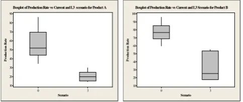
The designed flow process, the production schedule based on shipment date and the FIFO control systems are added to the current manufacturing system. After an implementation, it has been found that the results repeat the same as appeared on the computer simulation. The average of the production time per unit from Scenario L3 is lower than the current manufacturing system that describe in the figure of a box-whisker plot below (Fig. 9). Though there was the maintenance effect leading to the high variation of the production rates achieved from Product B.

Scenario

P

r

od

u

c

ti

on

R

a

te

3 0

90 80 70 60 50 40 30 20 10

Boxplot of Production Rate vs Current and L3 scenario for Product A

Scenario

P

r

od

u

c

ti

on

R

a

te

3 0

100 90 80 70 60 50 40 30 20 10

Boxplot of Production Rate vs Current and L3 Scenario for Product B

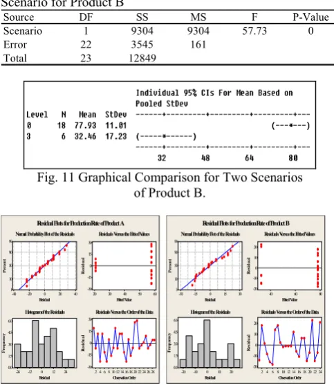
[image:5.595.307.549.552.654.2]

(6)

[image:6.595.47.290.229.369.2]

experimental results on all scenarios categorised by two types of products, A and B, were statistically significant with a 95% confidence interval (Tables 2 and 3). The numerical results suggested that Scenario L3 provided the better performance in terms of the average production rate (Figures. 10 and 11). The goodness of the linear statistical model via experimental errors or residuals is also adequate (Fig. 12). As the results, Scenario L3 is then applied to the manufacturing system under a consideration of the reduction of production time achieved [15].

TABLE 2 One-way ANOVA: Production Rate versus Scenario for Product A

Source DF SS MS F P-Value

Scenario 1 7920 7920 38.42 0

Error 27 5566 206

Total 28 13486

Fig. 10 Graphical Comparison for Two Scenarios of Product A.

TABLE 3 One-way ANOVA: Production Rate versus Scenario for Product B

Source DF SS MS F P-Value

Scenario 1 9304 9304 57.73 0

Error 22 3545 161

[image:6.595.45.287.390.669.2]

Total 23 12849

Fig. 11 Graphical Comparison for Two Scenarios of Product B.

Residual P ercen t 40 20 0 -20 -40 99 90 50 10 1 Fitted Value R es idua l 60 50 40 30 20 30 15 0 -15 -30 Residual F re que nc y 24 12 0 -12 -24 6.0 4.5 3.0 1.5 0.0 Observation Order R es idua l 28 26 24 22 20 18 16 14 12 10 8 6 4 2 30 15 0 -15 -30

Normal Probability Plot of the Residuals Residuals Versus the Fitted Values

Histogram of the Residuals Residuals Versus the Order of the Data

Residual Plots for Production Rate of Product A

Residual P ercen t 30 15 0 -15 -30 99 90 50 10 1 Fitted Value R es idua l 80 60 40 20 10 0 -10 -20 Residual F re q ue nc y 20 10 0 -10 -20 6.0 4.5 3.0 1.5 0.0 Observation Order Re si d u a l 24 22 20 18 16 14 12 10 8 6 4 2 20 10 0 -10 -20

Normal Probability Plot of the Residuals Residuals Versus the Fitted Values

Histogram of the Residuals Residuals Versus the Order of the Data

Residual Plots for Production Rate of Product B

Fig. 12 Model Adequacy Checking.

VI. CONCLUSIONS

The erbium doped fibre amplifier manufacturing process causes incapable production time to meet customers’ requirement with high levels of variation. Lean manufacturing systems providing various practical tools are then used to

develop the production line of the EDFA manufacturing processes. Moreover, computer simulation could be considered to help making a decision which lean concept alternatives will be the most efficient instead of applying directly to the real problem. The scenario with the highest levels of key performances will be implemented into the actual manufacturing process. From simulation results, a hybrid scenario of lean manufacturing systems leads to the better performance in terms of the mean production rate. The efficient designed process flow layout and the production schedule based on shipment date including the first in first out control systems are then implemented during a short period. It seems to improve the production rate, reduce the manufacturing cost and eliminate the current waste of EDFA manufacturing process when compared.

REFERENCES

[1] M. Pfennigbauer, P.J. Winzer, M.M. Strasser, and W.R. Leeb, "Optimum Optical and Electrical Filter Characteristics in Optically Preamplified Direct Detection (N) RZ Receivers, Proc. SPIE, Free-Space Laser Communication Technologies XIII, vol. 4272, 2001, pp. 160-169.

[2] E. Snoeks, G. N. van den Hoven and A. Polman, "Cooperative Up Conversion in Erbium-Implanted Soda-Lime Silicate Glass Optical

Waveguides," Journal of the Optical Society of America, vol. 12, no. 8,

1995, pp. 1468-1474 .

[3] N. Suthikarnnarunai, "Automotive Supply Chain and Logistics

Management," Proceedings of International MultiConference of

Engineers and Computer Scientists, Hong Kong,vol. 2, 2008.

[4] H. Czarnecki and N. Loyd, Simulation of Lean Assembly Line for High

Volume Manufacturing, "The Society for Modeling and Simulation

International", San Diego, 2001, pp. 1-6.

[5] Eng. Ana Rotaru, Implementing Lean Manufacturing, Technology in

Machine Building, The Annals of “DUNĂREA DE JOS” University of Galati Fascicle V, 2008.

[6] A. Mcleod, "Conceptual Development of an Introductory Lean Manufacturing, Course for Freshmen and Sophomore Level Students in Industrial Technology", the Technology Interface Journal/Fall, vol. 10 (1), 2009.

[7] A.D. Yablon, " Optical Fibre Fusion Splicing," Springer, 2004. [8] V. Modrák, Case on Manufacturing Cell Formation Using Production

Flow Analysis, International Journal of Mechanical, Industrial and

Aerospace Engineering, vol. 3(4), 2009, pp. 243–247.

[9] Y. Shi and M. Gregory, "International Manufacturing Networks - to

Develop Global Competitive Capabilities," Journal of Operations

Management, vol. 16, no. 2-3, 1998, pp. 195-214.

[10] W. D. Kelton, P. S. Randall, D. A. Sadowski, Simulation with Arena,

McGraw – Hill. Inc, 1998.

[11] A.J. Ruiz-Torres and K. Nakatani," Application of Real-Time

Simulation to Assign Due Dates on Logistic-Manufacturing Networks,"

The Winter Simulation Conference, 1998, pp. 1205-1210.

[12] T.T. Dimyati, "Minimising Production Flow Time in a Process and