Efficient Linearization of Tree Kernel Functions

Efficient Linearization of Tree Kernel Functions

Daniele Pighin

FBK-Irst, HLT

Via di Sommarive, 18 I-38100 Povo (TN) Italy pighin@fbk.eu

Alessandro Moschitti

University of Trento, DISI

Via di Sommarive, 14 I-38100 Povo (TN) Italy moschitti@disi.unitn.it

Abstract

The combination of Support Vector Machines with very high dimensional kernels, such as string or tree kernels, suffers from two ma-jor drawbacks: first, the implicit representa-tion of feature spaces does not allow us to un-derstand which features actually triggered the generalization; second, the resulting compu-tational burden may in some cases render un-feasible to use large data sets for training. We propose an approach based on feature space reverse engineering to tackle both problems. Our experiments with Tree Kernels on a Se-mantic Role Labeling data set show that the proposed approach can drastically reduce the computational footprint while yielding almost unaffected accuracy.

1 Introduction

The use of Support Vector Machines (SVMs) in supervised learning frameworks is spreading across different communities, including Computa-tional Linguistics and Natural Language Processing, thanks to their solid mathematical foundations, ef-ficiency and accuracy. Another important reason for their success is the possibility of using kernel functions to implicitly represent examples in some high dimensional kernel space, where their similar-ity is evaluated. Kernel functions can generate a very large number of features, which are then weighted by the SVM optimization algorithm obtaining a fea-ture selection side-effect. Indeed, the weights en-coded by the gradient of the separating hyperplane learnt by the SVM implicitly establish a ranking be-tween features in the kernel space. This property has been exploited in feature selection models based on

approximations or transformations of the gradient, e.g. (Rakotomamonjy, 2003), (Weston et al., 2003) or (Kudo and Matsumoto, 2003).

However, kernel based systems have two major drawbacks: first, new features may be discovered in the implicit space but they cannot be directly ob-served. Second, since learning is carried out in the dual space, it is not possible to use the faster SVM or perceptron algorithms optimized for linear spaces. Consequently, the processing of large data sets can be computationally very expensive, limiting the use of large amounts of data for our research or applica-tions.

We propose an approach that tries to fill in the gap between explicit and implicit feature represen-tations by 1) selecting the most relevant features in accordance with the weights estimated by the SVM and 2) using these features to build an explicit rep-resentation of the kernel space. The most innovative aspect of our work is the attempt to model and im-plement a solution in the context of structural ker-nels. In particular we focus on Tree Kernel (TK) functions, which are especially interesting for the Computational Linguistics community as they can effectively encode rich syntactic data into a kernel-based learning algorithm. The high dimensionality of a TK feature space poses interesting challenges in terms of computational complexity that we need to address in order to come up with a viable solution. We will present a number of experiments carried out in the context of Semantic Role Labeling, show-ing that our approach can noticeably reduce trainshow-ing time while yielding almost unaffected classification accuracy, thus allowing us to handle larger data sets at a reasonable computational cost.

The rest of the paper is structured as follows:

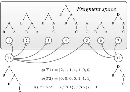
Fragment space

A B A

A B A

B A A B A

C A B A

B A C

A C

D B A

D B A

C

1 2 3 4 5 6 7

T1 A

B A B A

C

T2 D

B A C

φ(T1) = [2,1,1,1,1,0,0]

φ(T2) = [0,0,0,0,1,1,1]

K(T1, T2) =hφ(T1), φ(T2)i= 1

Figure 1: Esemplification of a fragment space and the kernel product between two trees.

tion 2 will briefly review SVMs and Tree Kernel functions; Section 3 will detail our proposal for the linearization of a TK feature space; Section 4 will review previous work on related subjects; Section 5 will describe our experiments and comment on their results; finally, in Section 6 we will draw our con-clusions.

2 Tree Kernel Functions

The decision function of an SVM is:

f(~x) =w~ _·~x+b=

n

X

i=1

αiyix~i·~x+b (1)

where ~xis a classifying example and w~ andb are

the separating hyperplane’s gradient and its bias, respectively. The gradient is a linear combination of the training points x~i, their labels yi and their

weights αi. These and the bias are optimized at

training time by the learning algorithm. Applying the so-calledkernel trickit is possible to replace the scalar product with a kernel function defined over pairs ofobjects:

f(o) =

n

X

i=1

αiyik(oi, o) +b

with the advantage that we do not need to provide an explicit mappingφ(·)of our examples in a vector space.

A Tree Kernel function is a convolution ker-nel (Haussler, 1999) defined over pairs of trees. Practically speaking, the kernel between two trees evaluates the number of substructures (orfragments) they have in common, i.e. it is a measure of their

overlap. The function can be computed recursively in closed form, and quite efficient implementations are available (Moschitti, 2006). Different TK func-tions are characterized by alternative fragment defi-nitions, e.g. (Collins and Duffy, 2002) and (Kashima and Koyanagi, 2002). In the context of this paper we will be focusing on the SubSet Tree (SST) ker-nel described in (Collins and Duffy, 2002), which relies on a fragment definition that does not allow to break production rules (i.e. if any child of a node is included in a fragment, then also all the other chil-dren have to). As such, it is especially indicated for tasks involving constituency parsed texts.

Implicitly, a TK function establishes a correspon-dence between distinct fragments and dimensions in somefragment space, i.e. the space of all the pos-sible fragments. To simplify, a treetcan be repre-sented as a vector whose attributes count the occur-rences of each fragment within the tree. The ker-nel between two trees is then equivalent to the scalar product between pairs of such vectors, as exempli-fied in Figure 1.

3 Mining the Fragment Space

If we were able to efficiently mine and store in a dictionary all the fragments encoded in a model, we would be able to represent our objects explicitly and use these representations to train larger models and very quick and accurate classifiers. What we need to devise are strategies to make this approach convenient in terms of computational requirements, while yielding an accuracy comparable with direct tree kernel usage.

Our framework defines five distinct activities, which are detailed in the following paragraphs. Fragment Space Learning (FSL) First of all, we can partition our training data into S smaller sets,

and use the SVM and the SST kernel to learnS

mod-els. We will use the estimated weights to drive our feature selection process. Since the time complexity of SVM training is approximately quadratic in the number of examples, this way we can considerably accelerate the process of estimating support vector weights.

minimization of the empirical risk (Vapnik, 1998). Nonetheless, since we do not need to employ them for classification (but just to direct our feature se-lection process, as we will describe shortly), we can accept to rely on sub-optimal weights. Furthermore, research results in the field of SVM parallelization using cascades of SVMs (Graf et al., 2004) suggest that support vectors collected from locally learnt models can encode many of the relevant features re-tained by models learnt globally. Henceforth, letMs

be the model associated with thes-th split, and_Fs

the fragment space that can describe all the trees in

Ms.

Fragment Mining and Indexing (FMI) In Equa-tion 1 it is possible to isolate the gradient w~ =

Pn

i=1αiyix~i, with x~i = [x(1)_i , . . . , x(_iN)], N being

the dimensionality of the feature space. For a tree kernel function, we can rewritex(_ij)as:

x(_ij) = ti,jλ

`(fj)

ktik

= ti,jλ`(fj)

qPN

k=1(ti,kλ`(fk))2

(2)

where:ti,j is the number of occurrences of the

frag-mentfj, associated with the j-th dimension of the

feature space, in the tree ti; λis the kernel decay

factor; and`(fj)is the depth of the fragment.

The relevance |w(j)_| of the fragment fj can be

measured as:

|w(j)|=

n

X

i=1

αiyix(_ij)

. (3)

We fix a threshold L and from each model Ms

(learnt during FSL) we select the L most relevant

fragments, i.e. we build the setFs,L=∪k{fk} so

that:

|Fs,L|=Land|w(k)| ≥ |w(i)|∀fi ∈ F \ Fs,L.

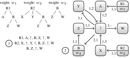
In order to do so, we need to harvest all the frag-ments with a fast extraction function, store them in a compact data structure and finally select the frag-ments with the highest relevance. Our strategy is ex-emplified in Figure 2. First, we represent each frag-ment as a sequence as described in (Zaki, 2002). A sequence contains the labels of the fragment nodes in depth-first order. By default, each node is the child of the previous node in the sequence. A spe-cial symbol (↑) indicates that the next node in the

R1 A B

Z W R2 X Y B

Z W B Z W weight:w1 weight:w2 weight:w3

R1, A,↑, B, Z,↑, W R2, X,↑, Y,↑, B, Z,↑, W

B, Z,↑, W

R1

w1

A

↑ W

X _wR2

2

Z Y

B

w3

1,1 1,2

2,1 1,1

1,1

1,-1,1 1,3 3,1

1,2

1

2

Figure 2: Fragment indexing. Each fragment is repre-sented as a sequence 1 _{and then encoded as a path in the} index 2 _{which keeps track of its cumulative relevance.}

sequence should be attached after climbing one level in the tree. For example, the tree(B (Z W))in figure is represented as the sequence[B, Z,↑, W]. Then, we add the elements of the sequence to a graph (which we call anindexof fragments) where each sequence becomes a path. The nodes of the index are the la-bels of the fragment nodes, and each arc is associ-ated with a pair of valueshd, n_i:dis a node identi-fier, which is unique with respect to the source node;

nis the identifier of the arc that must be selected at

the destination node in order to follow the path as-sociated with the sequence. Index nodes asas-sociated with a fragment root also have a field where the cu-mulative relevance of the fragment is stored.

As an example, the index node labeledB in fig-ure has an associated weight of w3, thus

identify-ing the root of a fragment. Each outgoidentify-ing edge univocally identifies an indexed fragment. In this case, the only outgoing edge is labeled with the pair

hd = 1, n = 1i, meaning that we should follow it to the next node, i.e.Z, and there select the edge la-beled1, as indicated byn. The edge withd= 1inZ

ishd= 1, n= 1i, so we browse to ↑where we se-lect the edgehd= 1, n=_−i. The missing value for ntells us that the next node,W, is the last element

of the sequence. The complete sequence is then[B, Z,↑, W], which encodes the fragment(B (Z W)).

The index implementation has been optimized for fast insertions and has the following features: 1) each node label is represented exactly once; 2) each distinct sequence tail is represented exactly once. The union of all the fragments harvested from each model is then saved into a dictionaryDLwhich will

be used by the next stage.

pro-Algorithm 3.1: MINE TREE(tree) global maxdepth, maxexp

main

mined← ∅;indexed← ∅;MINE(FRAG(tree),0)

procedureMINE(f rag, depth)

iff rag∈indexed

then return

indexed_←indexed_{∪ {}f rag_}

INDEX(f rag)

for eachnode_∈TO EXPAND(f rag)

do

  

ifnode6∈mined

then

mined_←mined_{∪ {}node_}

MINE(FRAG(node),0)

ifdepth < maxdepth

then

for eachf ragment∈EXPAND(f rag, maxexp)

doMINE(f ragment, depth+ 1)

cess by which tree nodes are included in a frag-ment. Fragment expansion is achieved vianode ex-pansions, where expanding a node means includ-ing its direct children in the fragment. The func-tion FRAG(n) builds the basic fragment rooted in a given noden, i.e. the fragment consisting only ofn

and its direct children. The functionTO EXPAND(f) returns the set of nodes in a fragment f that can

be expanded (i.e. internal nodes in the origin tree), while the functionEXPAND(f, maxexp) returns all the possible expansions of a fragment f. The

pa-rametermaxexpis a limit to the number of nodes

that can be expanded at the same time when a new fragment is generated, whilemaxdepthsets a limit

on the number of times that a base fragment can be expanded. The function INDEX(f) adds the frag-mentf to the index. To keep the notation simple,

here we assume that a fragment f contains all the

necessary information to calculate its relevance (i.e. the weight, label and norm of the support vectorαi,

yi, andktik, the depth of the fragment`(f)and the

decay factorλ, see equations 2 and 3).

Performing in a different order the same node ex-pansions on the same fragmentfresults in the same

fragmentf0. To prevent the algorithm from entering

circular loops, we use the set indexed so that the

very same fragment in each tree cannot be explored more than once. Similarly, the mined set is used

so that the base fragment rooted in a given node is considered only once.

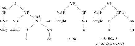
Tree Fragment Extraction (TFX) During this phase, a data file encoding label-tree pairshyi, tiiis

S NP NNP Mary

VP VB

bought

NP D

a

NN cat

(A1) (A0)

⇒

VP VB-P bought

NP D-B a

VP VB-P bought

NP-B D a

NN cat

-1: BC +1: BC,A1 -1: A0,A2,A3,A4,A5

Figure 3: Examples of ASTmstructured features. transformed to encode label-vector pairshyi, ~vii. To

do so, we generate the fragment space ofti, using

a variant of the mining algorithm described in Fig-ure 3.1, and encode inv~i all and only the fragments

ti,jso thatti,j ∈ DL, i.e. we perform feature

extrac-tion based on the indexed fragments. The process is applied to the whole training and test sets. The al-gorithm exploits labels and production rules found in the fragments listed in the dictionary to generate only the fragments thatmay bein the dictionary. For example, if the dictionary does not contain a frag-ment whose root is labeled N, then if a node N is

encountered during TFX neither its base fragment nor its expansions are generated.

Explicit Space Learning (ESL) After linearizing the training data, we can learn a very fast model by using all the available data and a linear kernel. The fragment space is nowexplicit, as there is a mapping between the input vectors and the fragments they en-code.

Explicit Space Classification (ESC) After learn-ing the linear model, we can classify our linearized test data and evaluate the accuracy of the resulting classifier.

4 Previous work

A rather comprehensive overview of feature selec-tion techniques is carried out in (Guyon and Elis-seeff, 2003). Non-filter approaches for SVMs and kernel machines are often concerned with polyno-mial and Gaussian kernels, e.g. (Weston et al., 2001) and (Neumann et al., 2005). Weston et al. (2003) use the`0 norm in the SVM optimizer to stress the

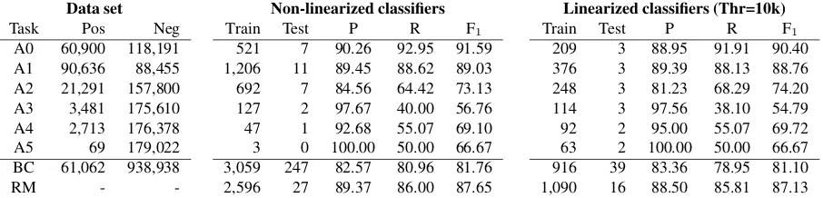
Data set Non-linearized classifiers Linearized classifiers (Thr=10k)

Task Pos Neg Train Test P R F1 Train Test P R F1

A0 60,900 118,191 521 7 90.26 92.95 91.59 209 3 88.95 91.91 90.40

A1 90,636 88,455 1,206 11 89.45 88.62 89.03 376 3 89.39 88.13 88.76

A2 21,291 157,800 692 7 84.56 64.42 73.13 248 3 81.23 68.29 74.20

A3 3,481 175,610 127 2 97.67 40.00 56.76 114 3 97.56 38.10 54.79

A4 2,713 176,378 47 1 92.68 55.07 69.10 92 2 95.00 55.07 69.72

A5 69 179,022 3 0 100.00 50.00 66.67 63 2 100.00 50.00 66.67

BC 61,062 938,938 3,059 247 82.57 80.96 81.76 916 39 83.36 78.95 81.10

RM - - 2,596 27 89.37 86.00 87.65 1,090 16 88.50 85.81 87.13

Table 1: Accuracy (P,R,F1), training (Train) and test (Test) time of non-linearized (center) and linearized (right)

classifiers. Times are in minutes. For each task, columnsPosandNeglist the number of positive and negative training examples, respectively. The accuracy of the role multiclassifiers is the micro-average of the individual classifiers trained to recognize core PropBank roles.

Suzuki and Isozaki (2005) present an embedded approach to feature selection for convolution ker-nels based on χ2-driven relevance assessment. To

our knowledge, this is the only published work clearly focusing on feature selection for tree ker-nel functions. In (Graf et al., 2004), an approach to SVM parallelization is presented which is based on a divide-et-impera strategy to reduce optimiza-tion time. The idea of using a compact graph rep-resentation to represent the support vectors of a TK function is explored in (Aiolli et al., 2006), where a Direct Acyclic Graph (DAG) is employed.

Concerning the use of kernels for NLP, inter-esting models and results are described, for exam-ple, in (Collins and Duffy, 2002), (Moschitti et al., 2008), (Kudo and Matsumoto, 2003), (Cumby and Roth, 2003), (Shen et al., 2003), (Cancedda et al., 2003), (Culotta and Sorensen, 2004), (Daum´e III and Marcu, 2004), (Kazama and Torisawa, 2005), (Kudo et al., 2005), (Titov and Henderson, 2006), (Moschitti et al., 2006), (Moschitti and Bejan, 2004) or (Toutanova et al., 2004).

5 Experiments

We tested our model on a Semantic Role La-beling (SRL) benchmark, using PropBank annota-tions (Palmer et al., 2005) and automatic Charniak parse trees (Charniak, 2000) as provided for the CoNLL 2005 evaluation campaign (Carreras and M`arquez, 2005). SRL can be decomposed into two tasks: boundary detection, where the word se-quences that are arguments of a predicate word w

are identified, androle classification, where each ar-gument is assigned the proper role. The former task requires a binaryBoundary Classifier(BC), whereas

the second involves a Role Multi-class Classifier

(RM).

Setup. If the constituency parse tree t of a

sen-tence s is available, we can look at all the pairs

hp, nii, where ni is any node in the tree and p is

the node dominatingw, and decide whetherniis an argument nodeor not, i.e. whether it exactly dom-inates all and only the words encoding any of w’s

arguments. The objects that we classify are sub-sets of the input parse tree that encompass both p

andni. Namely, we use the ASTm structure defined

in (Moschitti et al., 2008), which is the minimal tree that covers all and only the words ofp and ni. In

the ASTm,pandniare marked so that they can be

distinguished from the other nodes. An ASTm is

regarded as a positive example for BC ifniis an

ar-gument node, otherwise it is considered a negative example. Positive BC examples can be used to train an efficient RM: for each rolerwe can train a

clas-sifier whose positive examples are argument nodes whose label is exactlyr, whereas negative examples

are argument nodes labeled r0 ₆= r. Two ASTms

extracted from an example parse tree are shown in Figure 3: the first structure is a negative example for BC and is not part of the data set of RM, whereas the second is a positive instance for BC and A1.

To train BC we used PropBank sections 1 through 6, extracting ASTm structures out of the first 1

mil-lionhp, niipairs from the corresponding parse trees.

As a test set we used the 149,140 instance collected from the annotations in Section 24. There are 61,062 positive examples in the training set (i.e. 6.1%) and 8,515 in the test set (i.e. 5.7%).

1k 2k 5k 10k 20k30k 50k 100k

0 200 400 600 800 1,000 1,200

929 916 1,037

1,104

Threshold (log₁₀)

Learning

time

(minutes) _{Overall TFX ESL}

FMI FSL

Figure 4: Training time decomposition for the linearized BC with respect to its main components when varying the threshold value.

A5) from all the available training sections, i.e. 2 through 21, for a total of 179,091 training instances. Similarly, we collected 5,928 test instances from the annotations of Section 24.

In the remainder, we will mark with an`the

lin-earized classifiers, i.e. BC` and RM` will refer to

the linearized boundary and role classifiers, respec-tively. Their traditional, vanilla SST counterparts will be simply referred to as BC and RM.

We used 10 splits for the FMI stage and we set

maxdepth = 4andmaxexp = 5during FMI and TFX. We didn’t carry out an extensive validation of these parameters. These values were selected dur-ing the development of the software because, on a very small development set, they resulted in a very responsive system.

Since the main topic of this paper is the assess-ment of the efficiency and accuracy of our lineariza-tion technique, we did not carry out an evalualineariza-tion on the whole SRL task using the official CoNLL’05 evaluator. Indeed, producing complete annotations requires several steps (e.g. overlap resolution, OvA or Pairwise combination of individual role classi-fiers) that would shade off the actual impact of the methodology on classification.

Platform. All the experiments were run on a ma-chine equipped with 4 IntelR _XeonR _{CPUs clocked}

at 1.6 GHz and 4 GB of RAM running on a Linux 2.6.9 kernel. As a supervised learning framework we used SVM-Light-TK1_{, which extends the} SVM-Light optimizer (Joachims, 2000) with tree kernel

1_{http://disi.unitn.it/˜moschitt/Tree-Kernel.htm}

1k 2k 5k 10k 20k30k 50k 100k

72 74 76 78 80 82 84

Threshold (log₁₀)

Accurac

y

BC`Prec BC Prec

BC`Rec BC Rec

BC`F1 BC F1

Figure 5: BC`accuracy for different thresholds. support. During FSL, we learn the models using a normalized SST kernel and the default decay factor

λ = 0.4. The same parameters are used to train

the models of the non linearized classifiers. During ESL, the classifier is trained using a linear kernel. We did not carry out further parametrization of the learning algorithm.

Results. The left side of Table 1 shows the distri-bution of positive (ColumnPos) and negative (Neg) data points in each classifier’s training set. The cen-tral group of columns lists training and test effi-ciency and accuracy of BC and RM, i.e. the non-linearized classifiers, along with figures for the indi-vidual role classifiers that make up RM.

Training BC took more than two days of CPU time and testing about 4 hours. The classifier achieves an F1 measure of 81.76, with a good

bal-ance between precision and recall. Concerning RM, sequential training of the 6 models took 2,596 min-utes, while classification took 27 minutes. The slow-est of the individual role classifiers happens to be A1, which has an almost 1:1 ratio between posi-tive and negaposi-tive examples, i.e. they are 90,636 and 88,455 respectively.

We varied the threshold value (i.e. the number of fragments that we mine from each model, see Sec-tion 3) to measure its effect on the resulting classi-fier accuracy and efficiency. In this context, we call

training timeall the time necessary to obtain a lin-earized model, i.e. the sum of FSL, FMI and TFX time for every split, plus the time for ESL. Similarly, we calltest timethe time necessary to classify a lin-earized test set, i.e. the sum of TFX and ESC on test data.

learn-ing with respect to different threshold values. The Overall training time is shown alongside with par-tial times coming from FSL (which is the same for every threshold value and amounts to 433 minutes), FMI, training data TFX and ESL. The plot shows that TFX has a logarithmic behaviour, and that quite soon becomes the main player in total training time after FSL. For threshold values lower than 10k, ESL time decreases as the threshold increases: too few fragments are available and adding new ones in-creases the probability of including relevant frag-ments in the dictionary. After 10k, all the relevant fragments are already there and adding more only makes computation harder. We can see that for a threshold value of 100k total training time amounts to 1,104 minutes, i.e. 36% of BC. For a threshold value of 10k, learning time further decreases to 916 minutes, i.e. less than 30%. This threshold value was used to train the individual linearized role clas-sifiers that make up RM`.

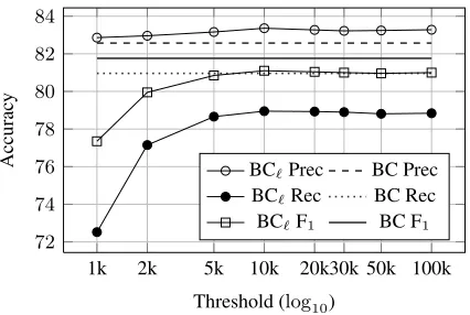
These considerations are backed by the trend of classification accuracy shown in Figure 5, where the Precision, Recall and F1 measure of BC`, evaluated

on the test set, are shown in comparison with BC. We can see that BC` precision is almost constant,

while its recall increases as we increase the thresh-old, reaches a maximum of 78.95% for a threshold of 10k and then settles around 78.8%. The F1 score

is maximized for a threshold of 10k, where it mea-sures 81.10, i.e. just 0.66 points less than BC. We can also see that BC` is constantly more

conserva-tive than BC, i.e. it always has higher precision and lower recall.

Table 1 compares side to side the accuracy (columns P, R and F1), training (Train) and test (Test) times of the different classifiers (central block of columns) and their linearized counterparts (block on the right). Times are measured in minutes. For the linearized classifiers, test time is the sum of TFX and ESC time, but the only relevant contribu-tion comes from TFX, as the low dimensional linear space and fast linear kernel allow us to classify test instances very efficiently2_{. Overall, BC}

`test time is

39 minutes, which is more than 6 times faster than BC (i.e. 247 minutes). It should be stressed that we

2_{Although ESC is not shown in table, the classification of all}

149k test instances with BC`took 5 seconds with a threshold of

1k and 17 seconds with a threshold of 100k.

Learning parallelization Task Non Lin. Linearized (Thr=10k)

1cpu 5cpus 10cpus

BC 3,059 916 293 215

RM 2,596 1,090 297 198

Table 2: Learning time when exploiting the framework’s parallelization capabilities. ColumnNon Lin. lists non-linearized training time.

are comparing against a fast TK implementation that is almost linear in time with respect to the number of tree nodes (Moschitti, 2006).

Concerning RM`, we can see that the accuracy

loss is even less than with BC`, i.e. it reaches an F1

measure of 87.13 which is just 0.52 less than RM. It is also interesting to note how the individual lin-earized role classifiers manage to perform accurately regardless of the distribution of examples in the data set: for all the six classifiers the final accuracy is in line with that of the corresponding non-linearized classifier. In two cases, i.e. A2 and A4, the accuracy of the linearized classifier is even higher, i.e. 74.20 vs. 73.13 and 69.72 vs. 69.10, respectively. As for the efficiency, total training time for RM` is 37% of

RM, i.e. 1,190 vs. 2,596 minutes, while test time is reduced to 60%, i.e. 16 vs 27 minutes. These improvements are less evident than those measured for boundary detection. The main reason is that the training set for boundary classification is much larger, i.e. 1 million vs. 179k instances: therefore, splitting training data during FSL has a reduced im-pact on the overall efficiency of RM`.

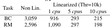
Parallelization. All the efficiency improvements that have been discussed so far considered a com-pletely sequential process. But one of the advan-tages of our approach is that it allows us to paral-lelize some aspect of SVM training. Indeed, every activity (but ESL) can exploit some degree of par-allelism: during FSL, all the models can be learnt at the same time (for this activity, the maximum de-gree of parallelization is conditioned by the number of training data splits); during FMI, models can be mined concurrently; during TFX, the data-set to be linearized can be split arbitrarily and individual seg-ments can be processed in parallel. Exploiting this possibility we can drastically improve learning ef-ficiency. As an example, in Table 2 we show how the total learning of the BC` can be cut to as low as

1 2 3 4 5 6 7 8 9 10 20

40 60 80 100

Models

Cumulati

ve

contrib

ution

(%)

1k 5k 10k

50k 100k

Figure 6: Growth of dictionary size when including frag-ments from more splits at different threshold values. When a low threshold is used, the contribution of indi-vidual dictionaries tends to be more marginal.

threshold of 10k. Even running on just 5 CPUs, the overall computational cost of BC`is less than 10%

of BC (Column Non Lin.). Similar considerations can be drawn concerning the role multi-classifier. Fragment space. In this section we take a look at the fragments included in the dictionary of the BC`

classifier. During FMI, we incrementally merge the fragments mined from each of the models learnt dur-ing FSL. Figure 6 plots, for different threshold val-ues, the percentage of new fragments (on theyaxis) that thei-th model (on thex axis) contributes with

respect to the number of fragments mined from each model (i.e. the threshold value).

If we consider the curve for a threshold equal to 100k, we can see that each model after the first ap-proximately contributes with the same number of fragments. On the other hand, if the threshold is set to 1k than the contribution of subsequent models is increasingly more marginal. Eventually, less than 10% of the fragments mined from the last model are new ones. This behaviour suggests that there is a core set of very relevant fragments which is com-mon across models learnt on different data, i.e. they are relevant for the task and do not strictly depend on the training data that we use. When we increase the threshold value, the new fragments that we index are more and more data specific.

The dictionary compiled with a threshold of 10k lists 62,760 distinct fragments. 15% of the frag-ments contain the predicate node (which generally is the node encoding the predicate word’s POS tag), more than one third contain the candidate argument

node and, of these, about one third are rooted in it. This last figure strongly suggests that the internal structure of an argument is indeed a very powerful feature not only for role classification, as we would expect, but also for boundary detection. About 10% of the fragments contain both the predicate and the argument node, while about 1% encode the Path fea-ture traditionally used in explicit semantic role label-ing models (Gildea and Jurafsky, 2002). About 5% encode a sort of extended Path feature, where the ar-gument node is represented together with its descen-dants. Overall, about 2/3 of the fragments contain at least some terminal symbol (i.e. words), generally a preposition or an adverb.

6 Conclusions

We presented a supervised learning framework for Support Vector Machines that tries to combine the power and modeling simplicity of convolution ker-nels with the advantages of linear kerker-nels and ex-plicit feature representations. We tested our model on a Semantic Role Labeling benchmark and ob-tained very promising results in terms of accuracy and efficiency. Indeed, our linearized classifiers manage to be almost as accurate as non linearized ones, while drastically reducing the time required to train and test a model on the same amounts of data.

To our best knowledge, the main points of nov-elty of this work are the following: 1) it addresses the problem of feature selection for tree kernels, ex-ploiting SVM decisions to guide the process; 2) it provides an effective way to make the kernel space observable; 3) it can efficiently linearize structured data without the need for an explicit mapping; 4) it combines feature selection and SVM parallelization. We began investigating the fragments generated by a TK function for SRL, and believe that study-ing them in more depth will be useful to identify new, relevant features for the characterization of predicate-argument relations.

References

Fabio Aiolli, Giovanni Da San Martino, Alessandro Sper-duti, and Alessandro Moschitti. 2006. Fast on-line kernel learning for trees. InProceedings of ICDM’06. Nicola Cancedda, Eric Gaussier, Cyril Goutte, and Jean Michel Renders. 2003. Word sequence kernels.

Journal of Machine Learning Research, 3:1059–1082. Xavier Carreras and Llu´ıs M`arquez. 2005. Introduction to the CoNLL-2005 Shared Task: Semantic Role La-beling. InProceedings of CoNLL’05.

Eugene Charniak. 2000. A maximum-entropy-inspired parser. InProceedings of NAACL’00.

Michael Collins and Nigel Duffy. 2002. New Rank-ing Algorithms for ParsRank-ing and TaggRank-ing: Kernels over Discrete Structures, and the Voted Perceptron. In Pro-ceedings of ACL’02.

Aron Culotta and Jeffrey Sorensen. 2004. Dependency Tree Kernels for Relation Extraction. InProceedings of ACL’04.

Chad Cumby and Dan Roth. 2003. Kernel Methods for Relational Learning. InProceedings of ICML 2003. Hal Daum´e III and Daniel Marcu. 2004. Np bracketing

by maximum entropy tagging and SVM reranking. In

Proceedings of EMNLP’04.

Daniel Gildea and Daniel Jurafsky. 2002. Automatic la-beling of semantic roles. Computational Linguistics, 28:245–288.

Hans P. Graf, Eric Cosatto, Leon Bottou, Igor Dur-danovic, and Vladimir Vapnik. 2004. Parallel support vector machines: The cascade svm. In Neural Infor-mation Processing Systems.

Isabelle Guyon and Andr´e Elisseeff. 2003. An intro-duction to variable and feature selection. Journal of Machine Learning Research, 3:1157–1182.

David Haussler. 1999. Convolution kernels on discrete structures. Technical report, Dept. of Computer Sci-ence, University of California at Santa Cruz.

T. Joachims. 2000. Estimating the generalization per-formance of a SVM efficiently. In Proceedings of ICML’00.

Hisashi Kashima and Teruo Koyanagi. 2002. Kernels for semi-structured data. InProceedings of ICML’02. Jun’ichi Kazama and Kentaro Torisawa. 2005. Speeding

up training with tree kernels for node relation labeling. InProceedings of HLT-EMNLP’05.

Taku Kudo and Yuji Matsumoto. 2003. Fast methods for kernel-based text analysis. InProceedings of ACL’03. Taku Kudo, Jun Suzuki, and Hideki Isozaki. 2005. Boosting-based parse reranking with subtree features. InProceedings of ACL’05.

Alessandro Moschitti and Cosmin Bejan. 2004. A se-mantic kernel for predicate argument classification. In

CoNLL-2004, Boston, MA, USA.

Alessandro Moschitti, Daniele Pighin, and Roberto Basili. 2006. Semantic role labeling via tree ker-nel joint inference. InProceedings of CoNLL-X, New York City.

Alessandro Moschitti, Daniele Pighin, and Roberto Basili. 2008. Tree kernels for semantic role labeling.

Computational Linguistics, 34(2):193–224.

Alessandro Moschitti. 2006. Making tree kernels prac-tical for natural language learning. InProccedings of EACL’06.

Julia Neumann, Christoph Schnorr, and Gabriele Steidl. 2005. Combined SVM-Based Feature Selection and Classification. Machine Learning, 61(1-3):129–150. Martha Palmer, Daniel Gildea, and Paul Kingsbury.

2005. The proposition bank: An annotated corpus of semantic roles.Comput. Linguist., 31(1):71–106. J. Pei, J. Han, Mortazavi B. Asl, H. Pinto, Q. Chen, U.

Dayal, and M. C. Hsu. 2001. PrefixSpan Mining Se-quential Patterns Efficiently by Prefix Projected Pat-tern Growth. InProceedings of ICDE’01.

Alain Rakotomamonjy. 2003. Variable selection using SVM based criteria. Journal of Machine Learning Re-search, 3:1357–1370.

Libin Shen, Anoop Sarkar, and Aravind k. Joshi. 2003. Using LTAG Based Features in Parse Reranking. In

Proceedings of EMNLP’06.

Jun Suzuki and Hideki Isozaki. 2005. Sequence and Tree Kernels with Statistical Feature Mining. In Proceed-ings of the 19th Annual Conference on Neural Infor-mation Processing Systems (NIPS’05).

Ivan Titov and James Henderson. 2006. Porting statisti-cal parsers with data-defined kernels. InProceedings of CoNLL-X.

Kristina Toutanova, Penka Markova, and Christopher Manning. 2004. The Leaf Path Projection View of Parse Trees: Exploring String Kernels for HPSG Parse Selection. InProceedings of EMNLP 2004.

Vladimir N. Vapnik. 1998. Statistical Learning Theory. Wiley-Interscience.

Jason Weston, Sayan Mukherjee, Olivier Chapelle, Mas-similiano Pontil, Tomaso Poggio, and Vladimir Vap-nik. 2001. Feature Selection for SVMs. In Proceed-ings of NIPS’01.

Jason Weston, Andr´e Elisseeff, Bernhard Sch¨olkopf, and Mike Tipping. 2003. Use of the zero norm with lin-ear models and kernel methods. J. Mach. Learn. Res., 3:1439–1461.