Pathologies of Neural Models Make Interpretations Difficult

Pathologies of Neural Models Make Interpretations Difficult

Shi Feng1 Eric Wallace1 Alvin Grissom II2 Mohit Iyyer3,4 Pedro Rodriguez1Jordan Boyd-Graber1

1_{University of Maryland}2_{Ursinus College}

3_{UMass Amherst}4_{Allen Institute for Artificial Intelligence}

{shifeng,ewallac2,entilzha,jbg}@umiacs.umd.edu,

agrissom@ursinus.edu,miyyer@cs.umass.edu

Abstract

One way to interpret neural model predic-tions is to highlight the most important in-put features—for example, a heatmap visu-alization over the words in an input sen-tence. In existing interpretation methods for

NLP, a word’s importance is determined by either input perturbation—measuring the de-crease in model confidence when that word is removed—or by the gradient with respect to that word. To understand the limitations of these methods, we use input reduction, which iteratively removes the least important word from the input. This exposes pathological be-haviors of neural models: the remaining words appear nonsensical to humans and are not the ones determined as important by interpreta-tion methods. As we confirm with human ex-periments, the reduced examples lack infor-mation to support the prediction of any la-bel, but models still make the same predic-tions with high confidence. To explain these counterintuitive results, we draw connections to adversarial examples and confidence cali-bration: pathological behaviors reveal difficul-ties in interpreting neural models trained with maximum likelihood. To mitigate their defi-ciencies, we fine-tune the models by encourag-ing high entropy outputs on reduced examples. Fine-tuned models become more interpretable under input reduction without accuracy loss on regular examples.

1 Introduction

Many interpretation methods for neural networks explain the model’s prediction as a counterfactual: how does the prediction change when the input is modified? Adversarial examples (Szegedy et al.,

2014; Goodfellow et al., 2015) highlight the in-stability of neural network predictions by showing how small perturbations to the input dramatically change the output.

SQUAD

Context In 1899, John Jacob Astor IV invested $100,000 for Tesla to further develop and produce a new lighting system. In-stead, Tesla used the money to fund his Colorado Springs experiments.

Original What did Tesla spend Astor’s money on ? Reduced did

Confidence 0.78→0.91

Figure 1: SQUAD example from the validation set. Given the originalContext, the model makes the same correct prediction (“Colorado Springs experiments”) on the Reduced question as the Original, with even higher confidence. For humans, the reduced question, “did”, is nonsensical.

A common, non-adversarial form of model in-terpretation is feature attribution: features that are crucial for predictions are highlighted in a heatmap. One can measure a feature’s importance by input perturbation. Given an input for text clas-sification, a word’s importance can be measured by the difference in model confidence before and after that word is removed from the input—the word is important if confidence decreases signifi-cantly. This is the leave-one-out method (Li et al.,

2016b). Gradients can also measure feature im-portance; for example, a feature is influential to the prediction if its gradient is a large positive value. Both perturbation and gradient-based methods can generate heatmaps, implying that the model’s pre-diction is highly influenced by the highlighted, im-portant words.

should match the leave-one-out method’s selec-tions, which closely align with human percep-tion (Li et al.,2016b;Murdoch et al.,2018). How-ever, rather than providing explanations of the original prediction, our reduced examples more closely resemble adversarial examples. In Fig-ure 1, the reduced input is meaningless to a hu-man but retains the same model prediction with high confidence. Gradient-based input reduction exposes pathological model behaviors that contra-dict what one expects based on existing interpreta-tion methods.

In Section2, we construct more of these coun-terintuitive examples by augmenting input reduc-tion with beam search and experiment with three tasks: SQUAD (Rajpurkar et al.,2016) for read-ing comprehension, SNLI (Bowman et al.,2015) for textual entailment, and VQA (Antol et al.,

2015) for visual question answering. Input re-duction with beam search consistently reduces the input sentence to very short lengths—often only one or two words—without lowering model confi-dence on its original prediction. The reduced ex-amples appear nonsensical to humans, which we verify with crowdsourced experiments. In Sec-tion3, we draw connections to adversarial exam-ples and confidence calibration; we explain why the observed pathologies are a consequence of the overconfidence of neural models. This elucidates limitations of interpretation methods that rely on model confidence. In Section 4, we encourage high model uncertainty on reduced examples with entropy regularization. The pathological model behavior under input reduction is mitigated, lead-ing to more reasonable reduced examples.

2 Input Reduction

To explain model predictions using a set of impor-tant words, we must first define importance. Af-ter defining input perturbation and gradient-based approximation, we describe input reduction with these importance metrics. Input reduction dras-tically shortens inputs without causing the model to change its prediction or significantly decrease its confidence. Crowdsourced experiments con-firm that reduced examples appear nonsensical to humans: input reduction uncovers pathological model behaviors.

2.1 Importance from Input Gradient

Ribeiro et al. (2016) and Li et al. (2016b) de-fine importance by seeing how confidence changes when a feature is removed; a natural approxima-tion is to use the gradient (Baehrens et al.,2010;

Simonyan et al.,2014). We formally define these importance metrics in natural language contexts and introduce the efficient gradient-based approx-imation. For each word in an input sentence, we measure its importance by the change in the con-fidence of the original prediction when we remove that word from the sentence. We switch the sign so that when the confidence decreases, the impor-tance value is positive.

Formally, letx=hx1, x2, . . . xnidenote the

in-put sentence,f(y|x)the predicted probability of labely, and y = argmax_y0f(y0|x) the original

predicted label. The importance is then

g(xi |x) =f(y|x)−f(y|x−i). (1)

To calculate the importance of each word in a sen-tence withnwords, we neednforward passes of the model, each time with one of the words left out. This is highly inefficient, especially for longer sentences. Instead, we approximate the impor-tance value with the input gradient. For each word in the sentence, we calculate the dot product of its word embedding and the gradient of the output with respect to the embedding. The importance of n words can thus be computed with a single forward-backward pass. This gradient approxima-tion has been used for various interpretaapproxima-tion meth-ods for natural language classification models (Li et al., 2016a; Arras et al., 2016); see Ebrahimi et al. (2017) for further details on the derivation. We use this approximation in all our experiments as it selects the same words for removal as an ex-haustive search (no approximation).

2.2 Removing Unimportant Words

Instead of looking at the words with high impor-tance values—what interpretation methods com-monly do—we take a complementary approach and study how the model behaves when the sup-posedly unimportant words are removed. Intu-itively, the important words should remain after the unimportant ones are removed.

experi-ment with three popular datasets: SQUAD ( Ra-jpurkar et al., 2016) for reading comprehension, SNLI (Bowman et al., 2015) for textual entail-ment, and VQA (Antol et al., 2015) for visual question answering. We describe each of these tasks and the model we use below, providing full details in the Supplement.

In SQUAD, each example is a context para-graph and a question. The task is to predict a span in the paragraph as the answer. We reduce only the question while keeping the context paragraph unchanged. The model we use is the DRQA Doc-ument Reader (Chen et al.,2017).

In SNLI, each example consists of two sen-tences: a premise and a hypothesis. The task is to predict one of three relationships: entailment, neutral, or contradiction. We reduce only the hy-pothesis while keeping the premise unchanged. The model we use is Bilateral Multi-Perspective Matching (BIMPM) (Wang et al.,2017).

In VQA, each example consists of an image and a natural language question. We reduce only the question while keeping the image unchanged. The model we use is Show, Ask, Attend, and An-swer (Kazemi and Elqursh,2017).

During the iterative reduction process, we en-sure that the prediction does not change (exact same span for SQUAD); consequently, the model accuracy on the reduced examples is identical to the original. The predicted label is used for input reduction and the ground-truth is never revealed. We use the validation set for all three tasks.

Most reduced inputs are nonsensical to humans (Figure2) as they lack information forany reason-able human prediction. However, models make confident predictions, at times even more confi-dent than the original.

To find the shortest possible reduced inputs (potentially the most meaningless), we relax the requirement of removing only the least impor-tant word and augment input reduction with beam search. We limit the removal to thek least impor-tant words, wherekis the beam size, and decrease the beam size as the remaining input is shortened.1 We empirically select beam size five as it pro-duces comparable results to larger beam sizes with reasonable computation cost. The requirement of maintaining model prediction is unchanged.

1_{We set beam size tomax(1,min(k, L−3))wherekis} maximum beam size andLis the current length of the input sentence.

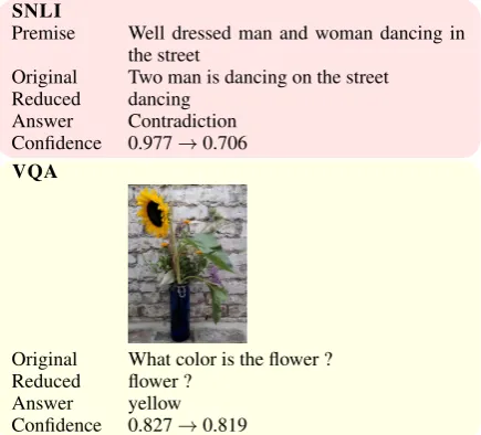
SNLI

Premise Well dressed man and woman dancing in the street

Original Two man is dancing on the street Reduced dancing

Answer Contradiction Confidence 0.977→0.706 VQA

Original What color is the flower ? Reduced flower ?

Answer yellow Confidence 0.827→0.819

Figure 2: Examples of original and reduced inputs where the models predict the sameAnswer. Reduced

shows the input after reduction. We remove words from the hypothesis for SNLI, questions for SQUAD and VQA. Given the nonsensical reduced inputs, humans would not be able to provide the answer with high con-fidence, yet, the neural models do.

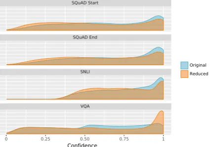
With beam search, input reduction finds ex-tremely short reduced examples with little to no decrease in the model’s confidence on its orig-inal predictions. Figure 3 compares the length of input sentences before and after the reduction. For all three tasks, we can often reduce the sen-tence to only one word. Figure 4 compares the model’s confidence on original and reduced in-puts. On SQUAD and SNLI the confidence

de-creases slightly, and on VQA the confidence even increases.

2.3 Humans Confused by Reduced Inputs

On the reduced examples, the models retain their original predictions despite short input lengths. The following experiments examine whether these predictions are justified or pathological, based on how humans react to the reduced inputs.

0 5 10 15 20 0

0.05 0.10 0.15 0.20

Frequency

11.5

2.3

Original Reduced Mean Length

0 5 10 15 20

7.5

1.5

0 5 10 15 20

Example Length

6.2

2.3

Figure 3: Distribution of input sentence length before and after reduction. For all three tasks, the input is often reduced to one or two words without changing the model’s prediction.

SQuAD Start

Original Reduced SQuAD End

SNLI

0 0.25 0.50 0.75 1

Confidence

VQA

Figure 4: Density distribution of model confidence on reduced inputs is similar to the original confidence. In SQUAD, we predict the beginning and the end of the answer span, so we show the confidence for both.

the correct answer, showing a significant accuracy loss on all three tasks (compareOriginaland Re-ducedin Table1).

The second setting examines how random the reduced examples appear to humans. For each of the original examples, we generate a version where words are randomly removed until the length matches the one generated by input reduc-tion. We present the original example along with the two reduced examples and ask crowd work-ers their preference between the two reduced ones. The workers’ choice is almost fifty-fifty (the vs. Randomin Table1): the reduced examples appear almost random to humans.

These results leave us with two puzzles: why are the models highly confident on the nonsensical reduced examples? And why, when the leave-one-out method selects important words that appear reasonable to humans, the input reduction process selects ones that are nonsensical?

Dataset Original Reduced vs. Random

SQUAD 80.58 31.72 53.70 SNLI-E 76.40 27.66 42.31 SNLI-N 55.40 52.66 50.64 SNLI-C 76.20 60.60 49.87 VQA 76.11 40.60 61.60

Table 1: Human accuracy onReducedexamples drops significantly compared to theOriginalexamples, how-ever, model predictions are identical. The reduced ex-amples also appear random to humans—they do not prefer them over random inputs (vs. Random). For SQUAD, accuracy is reported using F1 scores, other numbers are percentages. For SNLI, we report results on the three classes separately: entailment (-E), neutral (-N), and contradiction (-C).

3 Making Sense of Reduced Inputs

Having established the incongruity of our defini-tion of importance vis-`a-vis human judgements, we now investigate possible explanations for these results. We explain why model confidence can empower methods such as leave-one-out to gen-erate reasonable interpretations but also lead to pathologies under input reduction. We attribute these results to two issues of neural models.

3.1 Model Overconfidence

Neural models are overconfident in their predic-tions (Guo et al., 2017). One explanation for overconfidence is overfitting: the model overfits the negative log-likelihood loss during training by learning to output low-entropy distributions over classes. Neural models are also overconfident on examples outside the training data distribution. As

a human would trivially classify as not belonging to any class but for which the model predicts with high confidence. Goodfellow et al.(2015) argue that the rubbish examples exist for the same rea-son that adversarial examples do: the surprising linear nature of neural models. In short, the confi-dence of a neural model is not a robust estimate of its prediction uncertainty.

Our reduced inputs satisfy the definition of rub-bish examples: humans have a hard time making predictions based on the reduced inputs (Table1), but models make predictions with high confidence (Figure 4). Starting from a valid example, input reduction transforms it into a rubbish example.

The nonsensical, almost random results are best explained by looking at a complete reduction path (Figure 5). In this example, the transition from valid to rubbish happens immediately after the first step: following the removal of “Broncos”, humans can no longer determine which team the ques-tion is asking about, but model confidence remains high. Not being able to lower its confidence on rubbish examples—as it is not trained to do so— the model neglects “Broncos” and eventually the process generates nonsensical results.

In this example, the leave-one-out method will not highlight “Broncos”. However, this is not a failure of the interpretation method but of the model itself. The model assigns a low impor-tance to “Broncos” in the first step, causing it to be removed—leave-one-out would be able to expose this particular issue by not highlighting “Bron-cos”. However, in cases where a similar issue only appear after a few unimportant words are removed, the leave-one-out method would fail to expose the unreasonable model behavior.

Input reduction can expose deeper issues of model overconfidence and stress test a model’s un-certainty estimation and interpretability.

3.2 Second-order Sensitivity

So far, we have seen that the output of a neural model is sensitive to small changes in its input. We call thisfirst-ordersensitivity, because interpreta-tion based on input gradient is a first-order Taylor expansion of the model near the input (Simonyan et al., 2014). However, the interpretation also shifts drastically with small input changes (Fig-ure6). We call thissecond-ordersensitivity.

The shifting heatmap suggests a mismatch be-tween the model’s first- and second-order

sensi-SQUAD

Context: The Panthers used the San Jose State practice facility and stayed at the San Jose Marriott. The Broncos practiced at Stanford University and stayed at the Santa Clara Marriott.

Question:

(0.90, 0.89) Where did the Broncos practice for the Super Bowl ? (0.92, 0.88) Where did the practice for the Super Bowl ? (0.91, 0.88) Where did practice for the Super Bowl ? (0.92, 0.89) Where did practice the Super Bowl ? (0.94, 0.90) Where did practice the Super ? (0.93, 0.90) Where did practice Super ? (0.40, 0.50) did practice Super ?

Figure 5: A reduction path for a SQUAD validation ex-ample. The model prediction is always correct and its confidence stays high (shown on the left in parenthe-ses) throughout the reduction. Each line shows the in-put at that step with an underline indicating the word to remove next. The question becomes unanswerable im-mediately after “Broncos” is removed in the first step. However, in the context of the original question, “Bron-cos” is the least important word according to the input gradient.

tivities. The heatmap shifts when, with respect to the removed word, the model has low first-order sensitivity but high second-order sensitivity.

Similar issues complicate comparable interpre-tation methods for image classification models. For example, Ghorbani et al. (2017) modify im-age inputs so the highlighted features in the in-terpretation change while maintaining the same prediction. To achieve this, they iteratively mod-ify the input to maximize changes in the distribu-tion of feature importance. In contrast, the shift-ing heatmap we observe occurs by only remov-ing the least impactful features without a targeted optimization. They also speculate that the steep-est gradient direction for the first- and second-order sensitivity values are generally orthogonal. Loosely speaking, the shifting heatmap suggests that the direction of the smallest gradient value can sometimes align with very steep changes in second-order sensitivity.

When explaining individual model predictions, the heatmap suggests that the prediction is made based on a weighted combination of words, as in a linear model, which is not true unless the model is indeed taking a weighted sum such as in a DAN (Iyyer et al., 2015). When the model

SQUAD

Context: QuickBooks sponsored a “Small Business Big Game” contest, in which Death Wish Coffee had a 30-second commercial aired free of charge courtesy of QuickBooks. Death Wish Coffee beat out nine other contenders from across the United States for the free advertisement.

Question:

What company won free advertisement due to QuickBooks contest ? What company won free advertisement due to QuickBooks ? What company won free advertisement due to ?

What company won free due to ? What won free due to ? What won due to ? What won due to What won due What won What

Figure 6: Heatmap generated with leave-one-out shifts drastically despite only removing the least important word (underlined) at each step. For instance, “adver-tisement”, is the most important word in step two but becomes the least important in step three.

4 Mitigating Model Pathologies

The previous section explains the observed pathologies from the perspective of overconfi-dence: models are too certain on rubbish exam-ples when they should not make any prediction. Human experiments in Section 2.3 confirm that the reduced examples fit the definition of rubbish examples. Hence, a natural way to mitigate the pathologies is to maximize model uncertainty on the reduced examples.

4.1 Regularization on Reduced Inputs

To maximize model uncertainty on reduced ex-amples, we use the entropy of the output distri-bution as an objective. Given a modelf trained on a dataset(X,Y), we generate reduced exam-ples using input reduction for all training examexam-ples

X. Beam search often yields multiple reduced ver-sions with the same minimum length for each in-putx, and we collect all of these versions together to formX˜as the “negative” example set.

LetH(·)denote the entropy andf(y|x)denote

the probability of the model predictingygivenx. We fine-tune the existing model to simultaneously maximize the log-likelihood on regular examples and the entropy on reduced examples:

X

(x,y)∈(X,Y)

log(f(y|x)) +λX

˜ x∈X˜

H(f(y|x˜)),

(2) where hyperparameterλcontrols the trade-off be-tween the two terms. Similar entropy regulariza-tion is used by Pereyra et al. (2017), but not in

Accuracy Reduced length

Before After Before After

SQUAD 77.41 78.03 2.27 4.97 SNLI 85.71 85.72 1.50 2.20 VQA 61.61 61.54 2.30 2.87

Table 2: Model Accuracy on regular validation ex-amples remains largely unchanged after fine-tuning. However, the length of the reduced examples (Reduced length) increases on all three tasks, making them less likely to appear nonsensical to humans.

combination with input reduction; their entropy term is calculated on regular examples rather than reduced examples.

4.2 Regularization Mitigates Pathologies

On regular examples, entropy regularization does no harm to model accuracy, with a slight increase for SQUAD (Accuracyin Table2).

After entropy regularization, input reduction produces more reasonable reduced inputs (Fig-ure7). In the SQUAD example from Figure1, the reduced question changed from “did” to “spend Astor money on ?” after fine-tuning. The average length of reduced examples also increases across all tasks (Reduced length in Table 2). To verify that model overconfidence is indeed mitigated— that the reduced examples are less “rubbish” com-pared to before fine-tuning—we repeat the human experiments from Section2.3.

Human accuracy increases across all three tasks (Table 3). We also repeat thevs. Random exper-iment: we re-generate the random examples to match the lengths of the new reduced examples from input reduction, and find humans now pre-fer the reduced examples to random ones. The in-crease in both human performance and preference suggests that the reduced examples are more rea-sonable; model pathologies have been mitigated.

SQUAD

Context In 1899, John Jacob Astor IV invested $100,000 for Tesla to further develop and produce a new lighting system. In-stead, Tesla used the money to fund his Colorado Springs experiments.

Original What did Tesla spend Astor’s money on ? Answer Colorado Springs experiments

Before did

After spend Astor money on ? Confidence 0.78→0.91→0.52 SNLI

Premise Well dressed man and woman dancing in the street

Original Two man is dancing on the street Answer Contradiction

Before dancing After two man dancing Confidence 0.977→0.706→0.717 VQA

Original What color is the flower ? Answer yellow

Before flower ?

After What color is flower ? Confidence 0.847→0.918→0.745

Figure 7: SQUAD example from Figure1, SNLI and VQA (image omitted) examples from Figure2. We ap-ply input reduction to models bothBeforeandAfter en-tropy regularization. The models still predict the same

Answer, but the reduced examples after fine-tuning ap-pear more reasonable to humans.

5 Discussion

Rubbish examples have been studied in the image domain (Goodfellow et al., 2015; Nguyen et al.,

2015), but to our knowledge not forNLP. Our in-put reduction process gradually transforms a valid input into a rubbish example. We can often deter-mine which word’s removal causes the transition to occur—for example, removing “Broncos” in Figure5. These rubbish examples are particularly interesting, as they are also adversarial: the dif-ference from a valid example is small, unlike im-age rubbish examples generated from pure noise which are far outside the training data distribution. The robustness ofNLPmodels has been studied extensively (Papernot et al.,2016;Jia and Liang,

2017;Iyyer et al.,2018;Ribeiro et al.,2018), and most studies define adversarial examples similar to the image domain: small perturbations to the input lead to large changes in the output. Hot-Flip (Ebrahimi et al.,2017) uses a gradient-based approach, similar to image adversarial examples, to flip the model prediction by perturbing a few characters or words. Our work and Belinkov and Bisk (2018) both identify cases where noisy

Accuracy vs. Random

Before After Before After

SQUAD 31.72 51.61 53.70 62.75 SNLI-E 27.66 32.37 42.31 50.62 SNLI-N 52.66 50.50 50.64 58.94 SNLI-C 60.60 63.90 49.87 56.92 VQA 40.60 51.85 61.60 61.88

Table 3: HumanAccuracy increases after fine-tuning the models. Humans also prefer gradient-based re-duced examples over randomly rere-duced ones, indicat-ing that the reduced examples are more meanindicat-ingful to humans after regularization.

user inputs become adversarial by accident: com-mon misspellings break neural machine transla-tion models; we show that incomplete user input can lead to unreasonably high model confidence.

Other failures of interpretation methods have been explored in the image domain. The sensi-tivity issue of gradient-based interpretation meth-ods, similar to our shifting heatmaps, are observed by Ghorbani et al. (2017) and Kindermans et al.

(2017). They show that various forms of input perturbation—from adversarial changes to simple constant shifts in the image input—cause signifi-cant changes in the interpretation. Ghorbani et al.

(2017) make a similar observation about second-order sensitivity, that “the fragility of interpreta-tion is orthogonal to fragility of the predicinterpreta-tion”.

Previous work studies biases in the annotation process that lead to datasets easier than desired or expected which eventually induce pathological models. We attribute our observed pathologies primarily to the lack of accurate uncertainty es-timates in neural models trained with maximum likelihood. SNLI hypotheses contain artifacts that allowtraininga model without the premises ( Gu-rurangan et al., 2018); we apply input reduction at test time to the hypothesis. Similarly, VQA images are surprisingly unimportant for training a model; we reduce the question. The recent SQUAD 2.0 (Rajpurkar et al.,2018) augments the original reading comprehension task with an un-certainty modeling requirement, the goal being to make the task more realistic and challenging.

the model learns to minimize loss by outputting low-entropy distributions without improving vali-dation accuracy. To examine if overfitting can ex-plain the input reduction results, we run input re-duction using DRQA model checkpoints from ev-ery training epoch. Input reduction still achieves similar results on earlier checkpoints, suggesting that better convergence in maximum likelihood training cannot fix the issues by itself—we need new training objectives with uncertainty estima-tion in mind.

5.1 Methods for Mitigating Pathologies

We use the reduced examples generated by input reduction to regularize the model and improve its interpretability. This resembles adversarial train-ing (Goodfellow et al., 2015), where adversar-ial examples are added to the training set to im-prove model robustness. The objectives are dif-ferent: entropy regularization encourages high un-certainty on rubbish examples, while adversarial training makes the model less sensitive to adver-sarial perturbations.

Pereyra et al. (2017) apply entropy regulariza-tion on regular examples from the start of train-ing to improve model generalization. A similar method is label smoothing (Szegedy et al.,2016). In comparison, we fine-tune a model with entropy regularization on the reduced examples for better uncertainty estimates and interpretations.

To mitigate overconfidence, Guo et al. (2017) proposepost-hocfine-tuning a model’s confidence with Platt scaling. This method adjusts the soft-max function’s temperature parameter using a small held-out dataset to align confidence with ac-curacy. However, because the output is calibrated using the entire confidence distribution, not indi-vidual values, this does not reduce overconfidence on specific inputs, such as the reduced examples.

5.2 Generalizability of Findings

To highlight the erratic model predictions on short examples and provide a more intuitive demonstra-tion, we present paired-input tasks. On these tasks, the short lengths of reduced questions and hy-potheses obviously contradict the necessary num-ber of words for a human prediction (further sup-ported by our human studies). We also apply input reduction to single-input tasks including sentiment analysis (Maas et al.,2011) and Quizbowl ( Boyd-Graber et al.,2012), achieving similar results.

Interestingly, the reduced examples transfer to other architectures. In particular, when we feed fifty reduced SNLI inputs from each class—generated with the BIMPM model (Wang et al., 2017)—through the Decomposable Atten-tion Model (Parikh et al.,2016),2the same predic-tion is triggered 81.3% of the time.

6 Conclusion

We introduce input reduction, a process that it-eratively removes unimportant words from an in-put while maintaining a model’s prediction. Com-bined with gradient-based importance estimates often used for interpretations, we expose patholog-ical behaviors of neural models. Without lowering model confidence on its original prediction, an in-put sentence can be reduced to the point where it appears nonsensical, often consisting of one or two words. Human accuracy degrades when shown the reduced examples instead of the orig-inal, in contrast to neural models which maintain their original predictions.

We explain these pathologies with known is-sues of neural models: overconfidence and sen-sitivity to small input changes. The nonsensical reduced examples are caused by inaccurate uncer-tainty estimates—the model is not able to lower its confidence on inputs that do not belong to any label. The second-order sensitivity is another issue why gradient-based interpretation methods may fail to align with human perception: a small change in the input can cause, at the same time, a minor change in the prediction but a large change in the interpretation. Input reduction perturbs the input multiple times and can expose deeper issues of model overconfidence and oversensitivity that other methods cannot. Therefore, it can be used to stress test the interpretability of a model.

Finally, we fine-tune the models by maximizing entropy on reduced examples to mitigate the de-ficiencies. This improves interpretability without sacrificing model accuracy on regular examples.

To properly interpret neural models, it is impor-tant to understand their fundamental characteris-tics: the nature of their decision surfaces, robust-ness against adversaries, and limitations of their training objectives. We explain fundamental diffi-culties of interpretation due to pathologies in neu-ral models trained with maximum likelihood. Our

2_{http://demo.allennlp.org/}

work suggests several future directions to improve interpretability: more thorough evaluation of in-terpretation methods, better uncertainty and con-fidence estimates, and interpretation beyond bag-of-word heatmap.

Acknowledgments

Feng was supported under subcontract to Raytheon BBN Technologies by DARPA award HR0011-15-C-0113. JBG is supported by NSF Grant IIS1652666. Any opinions, findings, conclusions, or recommendations expressed here are those of the authors and do not necessarily reflect the view of the sponsor. The authors would like to thank Hal Daum´e III, Alexander M. Rush, Nicolas Papernot, members of the CLIP lab at the University of Maryland, and the anonymous reviewers for their feedback.

References

Stanislaw Antol, Aishwarya Agrawal, Jiasen Lu, Mar-garet Mitchell, Dhruv Batra, C. Lawrence Zitnick, and Devi Parikh. 2015. VQA: Visual question an-swering. InInternational Conference on Computer Vision.

Leila Arras, Franziska Horn, Gr´egoire Montavon, Klaus-Robert M¨uller, and Wojciech Samek. 2016. Explaining predictions of non-linear classifiers in NLP. InWorkshop on Representation Learning for

NLP.

David Baehrens, Timon Schroeter, Stefan Harmel-ing, Motoaki Kawanabe, Katja Hansen, and Klaus-Robert M¨uller. 2010. How to explain individual classification decisions. Journal of Machine Learn-ing Research.

Yonatan Belinkov and Yonatan Bisk. 2018. Synthetic and natural noise both break neural machine transla-tion. InProceedings of the International Conference

on Learning Representations.

Samuel R. Bowman, Gabor Angeli, Christopher Potts, and Christopher D. Manning. 2015. A large an-notated corpus for learning natural language infer-ence. InProceedings of Empirical Methods in

Nat-ural Language Processing.

Jordan L. Boyd-Graber, Brianna Satinoff, He He, and Hal Daum´e III. 2012. Besting the quiz master: Crowdsourcing incremental classification games. In

Proceedings of Empirical Methods in Natural Lan-guage Processing.

Danqi Chen, Adam Fisch, Jason Weston, and Antoine Bordes. 2017. Reading wikipedia to answer open-domain questions. InProceedings of the Association for Computational Linguistics.

Javid Ebrahimi, Anyi Rao, Daniel Lowd, and Dejing Dou. 2017. HotFlip: White-box adversarial exam-ples for text classification. InProceedings of the As-sociation for Computational Linguistics.

Amirata Ghorbani, Abubakar Abid, and James Y. Zou. 2017. Interpretation of neural networks is fragile.

arXiv preprint arXiv: 1710.10547.

Ian J. Goodfellow, Jonathon Shlens, and Christian Szegedy. 2015. Explaining and harnessing adver-sarial examples. InProceedings of the International

Conference on Learning Representations.

Chuan Guo, Geoff Pleiss, Yu Sun, and Kilian Q. Wein-berger. 2017. On calibration of modern neural net-works. InProceedings of the International Confer-ence of Machine Learning.

Suchin Gururangan, Swabha Swayamdipta, Omer Levy, Roy Schwartz, Samuel R. Bowman, and Noah A. Smith. 2018. Annotation artifacts in natural language inference data. InConference of the North American Chapter of the Association for Computa-tional Linguistics.

Mohit Iyyer, Varun Manjunatha, Jordan Boyd-Graber, and Hal Daum´e III. 2015. Deep unordered compo-sition rivals syntactic methods for text classification.

InProceedings of the Association for Computational

Linguistics.

Mohit Iyyer, John Wieting, Kevin Gimpel, and Luke S. Zettlemoyer. 2018. Adversarial example generation with syntactically controlled paraphrase networks.

InConference of the North American Chapter of the

Association for Computational Linguistics.

Robin Jia and Percy Liang. 2017. Adversarial ex-amples for evaluating reading comprehension sys-tems. InProceedings of Empirical Methods in

Nat-ural Language Processing.

Vahid Kazemi and Ali Elqursh. 2017. Show, ask, at-tend, and answer: A strong baseline for visual ques-tion answering. arXiv preprint arXiv: 1704.03162.

Pieter-Jan Kindermans, Sara Hooker, Julius Ade-bayo, Maximilian Alber, Kristof T. Sch¨utt, Sven D¨ahne, Dumitru Erhan, and Been Kim. 2017. The (un)reliability of saliency methods. arXiv preprint

arXiv: 1711.00867.

Jiwei Li, Xinlei Chen, Eduard H. Hovy, and Daniel Ju-rafsky. 2016a. Visualizing and understanding neural models in NLP. InConference of the North Amer-ican Chapter of the Association for Computational Linguistics.

Jiwei Li, Will Monroe, and Daniel Jurafsky. 2016b. Understanding neural networks through representa-tion erasure. arXiv preprint arXiv: 1612.08220.

Proceedings of the Association for Computational Linguistics.

W. James Murdoch, Peter J. Liu, and Bin Yu. 2018. Be-yond word importance: Contextual decomposition to extract interactions from lstms. InProceedings of the International Conference on Learning Represen-tations.

Anh Mai Nguyen, Jason Yosinski, and Jeff Clune. 2015. Deep neural networks are easily fooled: High confidence predictions for unrecognizable images.

InComputer Vision and Pattern Recognition.

Nicolas Papernot, Patrick D. McDaniel, Ananthram Swami, and Richard E. Harang. 2016. Crafting ad-versarial input sequences for recurrent neural net-works. IEEE Military Communications Conference.

Ankur P. Parikh, Oscar T¨ackstr¨om, Dipanjan Das, and Jakob Uszkoreit. 2016. A decomposable attention model for natural language inference. In Proceed-ings of Empirical Methods in Natural Language Processing.

Gabriel Pereyra, George Tucker, Jan Chorowski, Lukasz Kaiser, and Geoffrey E. Hinton. 2017. Reg-ularizing neural networks by penalizing confident output distributions. InProceedings of the

Interna-tional Conference on Learning Representations.

Pranav Rajpurkar, Robin Jia, and Percy Liang. 2018. Know what you don’t know: Unanswerable ques-tions for squad. In Proceedings of the Association for Computational Linguistics.

Pranav Rajpurkar, Jian Zhang, Konstantin Lopyrev, and Percy Liang. 2016. SQuAD: 100, 000+ questions for machine comprehension of text. InProceedings of Empirical Methods in Natural Language Process-ing.

Marco T´ulio Ribeiro, Sameer Singh, and Carlos Guestrin. 2016. Why should i trust you?”: Explain-ing the predictions of any classifier. InKnowledge

Discovery and Data Mining.

Marco Tulio Ribeiro, Sameer Singh, and Carlos Guestrin. 2018. Semantically equivalent adversar-ial rules for debugging nlp models. InProceedings of the Association for Computational Linguistics.

Karen Simonyan, Andrea Vedaldi, and Andrew Zisser-man. 2014. Deep inside convolutional networks: Vi-sualising image classification models and saliency maps. InProceedings of the International Confer-ence on Learning Representations.

Christian Szegedy, Vincent Vanhoucke, Sergey Ioffe, Jon Shlens, and Zbigniew Wojna. 2016. Rethinking the inception architecture for computer vision. In

Computer Vision and Pattern Recognition.

Christian Szegedy, Wojciech Zaremba, Ilya Sutskever, Joan Bruna, Dumitru Erhan, Ian J. Goodfellow, and Rob Fergus. 2014. Intriguing properties of neural

networks. InProceedings of the International Con-ference on Learning Representations.