Abstract— Imputation of missing data is important in many areas, such as reducing non-response bias in surveys and maintaining medical documentation. Estimating the uncertainty inherent in the imputed values is one way of evaluating the results of the imputation process. This paper presents a new method for the estimation of imputation uncertainty, which can be implemented as part of any imputation method, and which can be used to estimate the accuracy of the imputed values generated by both parametric and non-parametric imputation techniques. The proposed approach can be used to assess the feasibility of the imputation process for large complex datasets, and to compare the effectiveness of candidate imputation methods when they are applied to the same dataset. Current uncertainty estimation methods are described and their limitations are discussed. The ideas underpinning the proposed approach are explained in detail, and a case study is presented which shows how the new method has been applied in practice.
Index Terms— Imputation evaluation, Missing data,
Missingness patterns, Uncertainty estimation.
I. INTRODUCTION
Imputation methods attempt to solve the problem of missing data by replacing missing values with plausible estimates. Rubin [1] points outs that the primary (usually achievable) objective of imputation is to ensure that data analysis tools “can be applied to any dataset with missing values using the same command structure and output standards as if there were no missing data”, and that a further, desirable (but not always achievable) objective is to allow statistically valid inferences to be drawn when analysing imputed datasets. However, [2] also points out that “a popular misunderstanding is that the goal of imputation is to predict individual missing values”, and it is important to emphasise that imputed values should never be treated as if they are real values, since it is impossible to prove that they are accurate.
This complex definition of imputation objectives presents the owners of missing value datasets with complex evaluation problems, such as; How can the feasibility of the imputation project be assessed? How can the results of the imputation process be evaluated? How can the effectiveness of candidate
Manuscript received November 25, 2006.
The corresponding author is Norman Solomon: Tel.; +44-191-567-3382; e-mail: [email protected]
imputation methods be compared? We argue that these problems have not been sufficiently addressed, and we present a new method for the estimation and reduction of imputation uncertainty, which helps to solve them. The proposed approach can be implemented as part of any imputation method, and can be used to estimate the accuracy of the imputed values generated by both parametric and non-parametric imputation techniques.
Section II summarises current uncertainty estimation methods, and discusses their limitations. Section III explains the ideas underpinning the proposed method in detail. Section IV presents a case study which shows how the new method has been applied in practice. Section V summarises the paper and discusses the issues it raises.
II. CURRENT METHODS FOR ESTIMATING IMPUTATION UNCERTAINTY
Estimating the uncertainty inherent in the imputed values is one way of evaluating the results of the imputation process. Several methods for the estimation of imputation uncertainty have been proposed, and a good general overview of these can be found in [3]. The following sections summarise the most important methods, and discuss the limitations of these approaches.
A. Bootstrap and Jackknife Variance Estimation
Consider a variable Y =
(
y1,Kyn)
where some of thevalues are missing. The bootstrap and jackknife variance estimation methods [4]–[7] can be used to estimate the uncertainty created by imputing the missing values in Y. Where uncertainty is estimated by computing the variance of a set of parameter point estimates (such as the mean or standard deviation etc.), which describe a set of samples that are taken from Y, as follows;
for b = 1 to B
1. Create a new bootstrap sample Yb by randomly selecting a set of values (with replacement) from Y
2. Impute the missing values in Yb using a suitable imputation method
3. Compute a parameter point estimate θˆb which describes the values in Yb
next b
A Dynamic Method for the Evaluation and
Comparison of Imputation Techniques
The procedure produces a set of estimates {θˆ1KθˆB }
which describe the bootstrap samples {Y1KYB }. The
bootstrap estimate of the variance Vˆboot can then be used to
estimate imputation uncertainty, as follows;
(
)
∑
= − − = B b boot b boot B V 1 2 ˆ ˆ 1 1ˆ θ θ where
∑
= = B b b boot B 1 ˆ 1 ˆ θ θ
The method simply imputes the missing Yb values B times,
then computes the variance of the resulting set of
b
θˆ estimates. The jackknife variance estimation method is similar. The difference lies in the method used to create the set of samples, which in turn requires a more complex method of computing the variance, as follows;
Impute the missing values in Y using a suitable imputation method
Compute a parameter point estimate θˆwhich describes the values in
Y
for j = 1 to n
1. Delete value j from Y to create a new jackknife sample Y(\j)
2. Impute the missing values in Y(\j) using the same imputation method as above
3. Compute the same parameter estimate as above θˆ(\j) which describes the values in Y(\j)
next j
Where n is the number of values in Y =
(
y1,Kyn)
The procedure produces a set of estimates {
θ
ˆ(\1)Kθ
ˆ(\n)}which describe the jackknife samples {Y(\1)KY(\n)} The
jackknife estimate of the variance Vˆjack can then be used to estimate imputation uncertainty, as follows;
(
−)
∑
=(
−)
= n j jack j jack n n V 1 2 ˆ ~ 1 1ˆ
θ
θ
where
θ
~j =nθ
ˆ−(
n−1)
θ
ˆ(\j) and∑
= = n j j jack n 1 ~ 1 ˆθ
θ
The jackknife method can be much more computationally intensive than the bootstrap when n is large, since the imputation process must be repeated n times. However, in these cases jackknife performance can be improved by deleting a set of values (not just one) at each iteration of the loop.
B.Multiple Imputation
Consider a variable Y =
(
y1,Kyn)
where some of thevalues are missing. Multiple imputation (MI), [1] and [8]–[10] can be used to estimate the uncertainty created by imputing the missing values in Y, as follows.
for d = 1 to D
1. Impute the missing values in Y using a stochastic method to create a unique imputed dataset Yd
2. Compute a parameter point estimate θˆd which describes the values in Yd
3. Compute the variance Vd associated with θˆd next d
The procedure produces a set of estimates {θˆ1KθˆD } and a
set of associated variances {V1KVD } which describe the
imputed datasets {Y1KYD}. The combined MI complete-data
parameter point estimate for {Y1KYD } is then given by
∑
= = D d d D D 1 ˆ 1 θ θThe total variability TD, associated with θD, can then be
used to estimate imputation uncertainty, as follows;
(
)
⎟⎟ ⎠ ⎞ ⎜ ⎜ ⎝ ⎛ − − + + =∑
∑
= = D d D d D d d D D D D V D T 1 2 1 ˆ 1 1 11
θ
θ
It is important to emphasise that MI is primarily an imputation method, rather than a technique designed for the estimation of imputation uncertainty. However, “When the D sets of imputations are repeated random draws from the predictive distribution of the missing values under a particular model for nonresponse, the D complete-data inferences can be combined to form one inference that properly reflects uncertainty due to nonresponse under that model”, as succinctly explained in [3].
C.Limitations of Current Methods
The uncertainty estimation methods described above have their limitations, and they make certain assumptions about the nature of the missing value dataset. These issues have been the subject of some debate among statisticians [1] and [5]–[6]. The main points for discussion are summarised below.
• All of the methods described above assume that the imputation process has removed the bias within the dataset that was caused by the missing values [3]. • The resampling methods described in section IIA are
based on large-sample theory - i.e. they will return more reliable variance estimates for larger samples [3]. • The MI method assumes that the model describing the
• Resampling methods usually require several hundred executions of the imputation process, performed against an equal number of samples drawn from the missing value dataset. This can be impractical in some situations. However, MI is less computationally intensive, since it allows good inferences to be drawn for a wide range of estimands, using perhaps 10 (or less) imputed datasets [12].
• The methods described above make no provision for the reduction of imputation uncertainty. However, there seems to be no reason why they could not be adapted for this purpose.
The following section presents a new method for the estimation and reduction of imputation uncertainty, which suffers from none of the above limitations. However, the proposed approach has its own limitations, and makes its own assumptions, which are also described below.
III. ADYNAMIC METHOD FOR ESTIMATING AND REDUCING IMPUTATION UNCERTAINTY
Consider a data matrix Y which has one or more missing values in one or more of it’s columns, such as the matrix shown below. ⎥ ⎥ ⎥ ⎥ ⎥ ⎥ ⎥ ⎥ ⎦ ⎤ ⎢ ⎢ ⎢ ⎢ ⎢ ⎢ ⎢ ⎢ ⎣ ⎡ − − − − − − − − − − − − − − − − − − − = ? ? ? ? ? ? ? ? ? ? ? Y
The missing values are represented by ? symbols. The known values are represented by – symbols. The rows are indexed as i = 1 to n
[image:3.612.339.561.141.305.2]The columns are indexed as j = 1 to p Rows 1 and 4 have missingness pattern 10101 Rows 2 and 6 have missingness pattern 10011
Fig. 1 – Missingness patterns in a data matrix
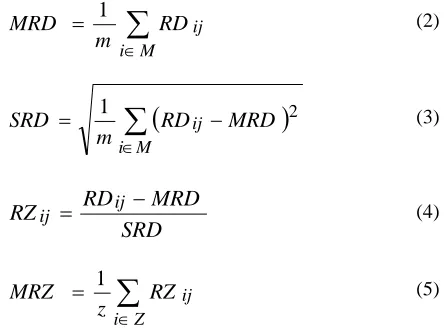
A small proportion (perhaps up to 10%) of the known values are deleted at random from within the variable (column in Y) to be imputed. These values are recorded just before they are deleted, and a measure of how accurately they have been “put back” is taken when the imputation process is complete. This basic technique (with appropriate modifications) has been frequently employed to evaluate the success of various new, and existing, imputation methods [13]–[16], but it has not been utilised as a technique for the estimation and reduction of imputation uncertainty. However, the following equations can be used to estimate imputation uncertainty when this evaluation technique is employed.
ij
RD
=trueVal Y imputedVal Y trueVal Y ij ij ij . . . − (1)
Where Yij.trueVal is the known (true) value that was
deleted. And Yij.imputedVal is the value generated by the
imputation process.
∑
∈ = M i ij RD mMRD 1 (2)
(
)
∑
∈ − = M i ij MRD RD mSRD 1 2 (3)
SRD MRD RD
RZij = ij − (4)
∑
∈ = Z i ij RZ zMRZ 1 (5)
Where j is the column in the Y matrix from which the values were randomly deleted and “put back”. And
} ,.... {r1 rm
M = is the set of rows in Y with a deleted value. And i indexes the set of rows in M (which will differ for every execution of the method). And Z = {r1,.... rz} is the set of rows in Y that have an RD outlier value.
The RD gives the relative differences between the known (true) and imputed values in column j of Y. The MRD gives the mean RD value - where larger MRD values indicate greater imputation uncertainty within the set of imputed values. The
SRD gives the standard deviation of the RD - where larger
SRD values indicate greater variability of the uncertainty. Values of RZ within any required range, such as ±3
SRD’s above and below the MRD, define RD outliers. Essentially, the RZ is a measure of the number of SRD’s by which any particular value of RD deviates from the MRD - where the set of RD values are assumed to be approximately normally distributed for this purpose. The MRZ gives the mean
RZ value - where PZ = z / m gives the proportion of RD outliers found within the set M.
variable to be imputed increases the proportion of missing data in that variable. This affects the results of the imputation process, since more values need to be imputed. Further, since the method deletes values completely at random, it is assumed that the truly missing values (unknown values, rather than known values which have been deleted) are also missing completely at random (MCAR), in the rigorous sense defined in [17]. However, the MCAR assumption can never be proved or disproved, regardless of the uncertainty estimation method used, because it is impossible to find any sort of pattern within a set of unknown values, as pointed out in [18].
A.Estimating Uncertainty by Segmenting the Dataset
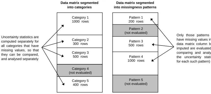
Generally, larger MRD values indicate greater uncertainty within the set of imputed values. However, larger SRD values show that this uncertainty is highly variable, and therefore it may be localised within one or more clearly defined data segments within the variable to be imputed - such as a particular set of missingness patterns (see Fig. 1), or a set of categories with clearly defined boundaries. In these cases it can be useful to discover the distribution of the RD values across these data segments, or to discover whether some segments contain higher proportions of RD outlier values than others (using equations (4) and (5)). To achieve this it is essential to delete the same proportion of values from each segment before measuring the uncertainties, so that each segment can be assessed equally.
Segmentation by category can be used to estimate the uncertainty created by imputation methods which do not utilise the missingness patterns within the data matrix - e.g. those methods which do not rely on regression based techniques to generate imputed values. When the dataset is segmented by category the process of deleting the same proportion of values from each category can be easily achieved by detecting the first and last rows of each category within the data matrix, as shown
in the left hand part of Fig. 2, below. However, it should be ensured that the proportion of known values in each category is sufficient to support the imputation process (where this is required - depending on the imputation method used, and on the proportion of truly missing values in each category). In cases where this is not possible the offending categories should be excluded from the uncertainty estimation process.
The method can also be used to compare and analyse the uncertainties within the missingness patterns found in the data matrix, as shown in the right hand part of Fig. 2. This can be implemented as part of any regression based imputation method which derives a different set of regression coefficients for each missingness pattern.
For example, the expectation-maximisation (EM) imputation algorithm, as described in [19] and [20], estimates missing values by deriving a unique regression equation for each row within each missingness pattern. Where each term in this equation is formed using the product of one of the derived regression coefficients for the missingness pattern in question, and one of the known values in the row being imputed. However, if the known values within a particular pattern do not form any sort of order within themselves (if they cannot be used to predict one another), then the uncertainty within the imputed values in this pattern will be large.
[image:4.612.87.518.499.692.2]To properly compare and analyse the uncertainty within the imputed values in each missingness pattern it is essential to delete the same proportion of known values from all of the patterns to be evaluated. The algorithm used to perform these deletions must ensure that deleting values from the variable to be imputed does not create any new (and hence artificial) missingness patterns within the data matrix. A description of this algorithm, which is the most procedurally complex part of the proposed approach, is given below.
Fig. 2 – Comparing and analysing the uncertainty in different data segments
Pattern 1 200 rows Pattern 2 (not evaluated)
Pattern 3 500 rows
Pattern 4 1000 rows
Pattern 5 (not evaluated)
Data matrix segmented into missingness patterns
Category 1 1000 rows
Category 2 300 rows
Category 5 400 rows Category 3 500 rows
Data matrix segmented into categories
Category 4 (not evaluated) Uncertainty statistics are
computed separately for all categories that have missing values, so that they can be compared, and analysed separately
function matrix balanced_ random_deletion_across_all_missingness_patterns_in_the_data_matrix ( matrix data, vector patterns, int c, int d ) dataMatrixRow data_row
vector match_rows missPatternRow patt
integer rows_to_add, random_row boolean match
for i = 1 to num_rows_in ( patterns ) patt = patterns ( i )
if ( patt ( c ) == missing && some_values_are_present_in ( patt ) == true ) match_rows = new vector ( )
for k = 1 to num_rows_in ( data ) data_row = data ( k ) if ( data_row ( c ) == present ) match = true
for j = 1 to num_columns_in ( data )
if ( patt ( j ) == present && data_row ( j ) == missing ) match = false
end if next j if ( match == true )
match_rows . Add_To_End ( k ) end if
end if next k
rows_to_add = ( d / 100 ) * num_rows_in ( patt ) if ( num_rows_in ( match_rows ) > rows_to_add * 2 ) for k = 1 to rows_to_add
random_row = Random ( 1, num_rows_in ( match_rows ) ) data_row = data ( match_rows ( random_row ) )
match_rows . Remove_Row ( random_row ) for j = 1 to num_columns_in ( data ) if ( patt ( j ) == missing ) data_row ( j ) = missing
end if next j next k end if
end if next i return data
end function
Algorithm 1 – A procedure to perform balanced random deletions across a set of missingness patterns The procedure increases the number of rows in each of the
missingness patterns to be evaluated by the same proportion, i.e. the number of rows in each pattern that has missing values in column c is increased by d%. This is achieved by transferring
data matrix rows from one pattern to another. For example, when deleting from data column one the procedure might transfer a data row by changing it’s pattern from “1111” to “0111”. However, the data rows transferred must have known values in the same columns as the data rows in the pattern to be evaluated (the pattern with rows added to it). For example, if the pattern to be evaluated was “0011”, then data rows with the pattern “1100” could not be transferred to that pattern, but
data rows with the pattern “1111”, could be transferred to it. The final pair of nested for loops perform the random row
B.Reducing Imputation Uncertainty
The method described in the preceding section allows the uncertainty in each data segment (see Fig. 2) to be estimated separately - i.e. the method allows the statistics returned by equations (1) to (5) to be computed separately for each segment. Further, since the same proportion of values were deleted from each segment, an additional uncertainty statistic can be computed for each segment, as follows;
Let j = the column in the Y matrix from which the values were randomly deleted and “put back”.
Let D = the data segment being evaluated for uncertainty (see Fig. 2).
Let
S
=
{
r
1,....
r
s}
be the set of rows in D with a deleted value, where i indexes these rows.Let M ={r1,....rm} be the set of all rows in Y with a deleted value, where i indexes these rows
The expected uncertainty for the data segment D is then given by
∑
∈ =
M i
ij
RD m
s EU
Where each RDij value is computed using equation (1)
The expected uncertainty is simply a device which enables the calculation of a useful uncertainty statistic. In fact, one would expect the uncertainty within the imputed values in each segment to be very different, rather than conforming to some expected value. For example, one would expect the regression equations derived for each missingness pattern to have different predictive powers. Therefore, one would expect the imputed values generated using these equations to have varying degrees of uncertainty. However, the idea is to use the notion of the expected uncertainty to compute the statistic described below. This is achieved by comparing the expected and actual uncertainties for the data segment D, where the actual uncertainty is given by
∑
∈ =
S i
ij
RD AU
Where each RDij value is computed using equation (1)
It follows that the equation SU = AU EU can be used to discover whether the data segment D has contributed more or less than it’s expected proportion of the overall uncertainty within the imputed values in column j of the Y data matrix. For example,
If SU = 0.5 then D has contributed half of it’s expected proportion of the overall uncertainty.
If SU = 10 then D has contributed ten times it’s expected proportion of the overall uncertainty.
Consequently, all of the data segments which contribute
more than their expected share of the overall uncertainty can be discovered. The MRD and SU for each segment can then be used to estimate the uncertainty in those segments. And in cases where the uncertainty for a particular segment is disproportionately large, the overall uncertainty can be reduced by discarding all of the imputed values in that segment. This approach can be beneficial in cases where the proportion of imputed values in the offending segments is relatively small - i.e. in these cases the overall uncertainty will be reduced by discarding a small proportion of the imputed values. However, in cases where the proportion of imputed values in the offending segments is relatively large, a much larger proportion of the imputed values would be discarded - and in the most extreme cases the best decision could be not to proceed with the imputation process at all.
The fundamental argument underpinning this method of uncertainty reduction is as follows. If the deleted values in a particular segment were “put back” very inaccurately, then it is probable that the truly missing values in this segment will contain imputation errors of a similar magnitude. However, it is impossible to prove, or disprove, this assertion, because the imputation of truly missing values can never be proven to be accurate using any approach - since the true values are unavailable for comparison.
It is important to emphasise that the decision to discard the imputed values in a particular data segment must be taken by the user of the imputation software. This decision is complex and difficult to automate, because all of the uncertainty statistics for all of the segments need to be considered and compared. For example, an examination of the uncertainty statistics could reveal that the uncertainty in a particular segment has been caused by one or two extreme outlier RD
values (see equations (4) and (5)). In such cases the user of the software might decide to examine the data rows in the offending segment in detail, to discover why this has occurred. This could reveal some hidden characteristics of the missing value dataset, which could not be discovered using any other approach.
Table I – Variables in the case study dataset
Dataset variable % missing
UKSIC Category 0 % OS Easting 0 % OS Northing 0 % Number of Employees 0 %
Payroll 63.08 % Sales 67.50 % Net Worth 40.69 %
Profit Before Tax 58.16 % Directors Pay 59.40 %
Depreciation 63.90 %
• The financial variables all have large proportions of missing data.
• 39% of the SME’s have no known financial figures whatsoever.
• The known values within the financial variables contain small proportions of extreme outlier values.
• There are 24 missingness patterns within the dataset, but these are unbalanced, with some patterns containing very few SME’s.
• There are 479 different UKSIC categories within the dataset, but approximately 11% of these have more than 80% missing values.
• The quality of the UKSIC categorization is poor, with some categories containing SME’s that could not be properly classified.
Where the SME’s in each UKSIC (United Kingdom Standard Industrial Classification) category carry out the same commercial activities, such as “Publishing of software” etc. And where the OS Easting and OS Northing variables specify the geographical location of each SME, using UK Ordnance Survey mapping co-ordinates.
The imputation experiments described below were designed to discover whether imputation of the missing financial figures was feasible, and to discover whether a parametric imputation method (the EM algorithm) or a non-parametric imputation method (K nearest neighbors (KNN), [15], [16] and [21]) would produce the least uncertainty within the imputed values. For EM imputation a matrix was formed (see Fig. 1) with 61,389 rows and 7 columns - i.e. the 6 SME financial variables and the number of employees. The EM algorithm was then used to impute all of the missing values in the matrix using a single execution of that algorithm. The following distance function was employed for nearest neighbor imputation
(
)
(
)
∑
∑
= =
= k
i
k
i m i i
m i m
S S d S
S d
donorVal S
imputedVal S
1 1 ,
1 ,
. .
Where Sm is the SME with the missing financial value, and i
S are the set of k nearest neighbor SME’s (donors), which are taken from the same UKSIC category as Sm, and which
have the same (or the closest available) number of employees as Sm And where d
(
Sm,Si)
gives the geographical(Euclidean) distance between Sm and Si , so that financial
values in geographically closer SME donors are given more weight.
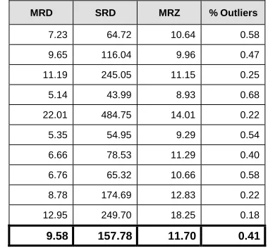
[image:7.612.341.532.255.431.2]The results of the Payroll imputation evaluation experiments are tabulated below - i.e. Tables II and III show the uncertainty statistics that were produced (using equations (1) to (5)) when imputing the missing Payroll figures for 61,389 SME’s, using the EM and KNN imputation methods described above.
Table II – Evaluation of the EM imputation process.
MRD SRD MRZ % Outliers
6.75 97.03 14.22 0.27 5.65 67.13 14.01 0.32 6.50 55.34 8.63 0.80 7.13 65.20 8.92 0.75 6.22 67.29 10.78 0.48 5.29 57.01 11.38 0.43 3.85 30.68 7.68 0.91 8.92 111.07 10.76 0.54 7.38 76.39 9.23 0.70 7.35 93.14 11.02 0.37
6.50 72.03 10.66 0.56
Table III – Evaluation of the KNN imputation process.
MRD SRD MRZ % Outliers
7.23 64.72 10.64 0.58 9.65 116.04 9.96 0.47 11.19 245.05 11.15 0.25 5.14 43.99 8.93 0.68 22.01 484.75 14.01 0.22 5.35 54.95 9.29 0.54 6.66 78.53 11.29 0.40 6.76 65.32 10.66 0.58 8.78 174.69 12.83 0.22 12.95 249.70 18.25 0.18
9.58 157.78 11.70 0.41
A. Interpreting the Experimental Results
[image:7.612.342.532.473.649.2]of the uncertainty statistics produced could be considered. The bottom rows of Tables II and III give the mean values of the statistics produced for all 20 experiments. A reasonable uncertainty benchmark for any imputation process would be an MRD value of less than one - i.e. the deleted values should be “put back” (on average) to within 100% of their true values. However, Tables II and III show that the MRD values returned for the SME dataset were 6.50 (for the EM imputation process) and 9.58 (for KNN) - i.e. the expected high uncertainty levels appeared, because of the overall poor quality of the data.
The MRD values in Table II show that the EM imputation process created less uncertainty than the KNN process, and the SRD values show that EM also produced less variable uncertainty than KNN - i.e. the uncertainty for the KNN process was much more dependant on the particular set of values that were deleted. The MRZ and % Outliers show that a small proportion of the deleted values were “put back” very inaccurately for every experiment. Further investigation revealed that these inaccurately replaced values were causing the major portion of the uncertainty - i.e. equation (1) returned RD values of between zero and one for at least 83% of the deleted values for every experiment, but the MRD values were always much larger, as Tables II and III show.
For EM, the same two missingness patterns were found to be causing the major portion of the overall uncertainty for every experiment. However, these patterns contained most of the SME’s, and discarding the imputed values in them would have removed over 80% of the imputed values, so this was not attempted. For KNN the UKSIC categories causing the most uncertainty differed for every experiment - i.e. they depended on the particular set of values that were deleted - so there was no point in discarding the imputed values in any of these categories.
It was therefore concluded that the high proportion of missing Payroll values, combined with the overall poor quality of the dataset, made the feasibility of Payroll imputation questionable, and that in this case discarding the imputed values in selected data segments could not be effectively used to decrease imputation uncertainty. It was further concluded that if imputation was to be attempted, a parametric method should be used, but the simple EM method described above should be improved. For example, the missing values within each UKSIC category could be imputed separately, and some way of utilising the geographical information could be built into the process.
V. SUMMARY AND DISCUSSION
How can the feasibility of the imputation project be assessed? How can the results of the imputation process be evaluated? How can the effectiveness of candidate imputation methods be compared? We argue that these problems have not been sufficiently addressed, and we have presented a new method for the estimation and reduction of imputation uncertainty, which helps to solve them. All imputation methods have the
same basic objective - i.e. they try to make the best possible use of the information content (the patterns etc.) within the known
values, to generate the best possible estimates for the missing
values. We argue that uncertainty evaluation methods should also make the best possible use of the known values, and the method described in this paper does just this.
Current uncertainty estimation methods have their limitations. In particular, they take no account of the accuracy of the imputed values, and they make no provision for the reduction of imputation uncertainty. The proposed approach addresses these problems, and we argue that the new method is fully consistent with imputation objectives, since it would be very hard to deny the success of any imputation method which can be shown to have repeatedly “put back” a set deleted values with a high degree of accuracy.
The proposed approach allows the uncertainty within different data segments (such as missingness patterns) to be estimated separately. And in cases where the uncertainty for a particular segment is disproportionately large, the overall uncertainty can be reduced by discarding all of the imputed values in that segment. Current uncertainty estimation methods do not adopt this approach, but there seems to be no reason why they could not be adapted for this purpose. However, is important to emphasise that the decision to discard the imputed values in a particular segment must be taken by the user of the imputation software. We argue that there is no substitute for human judgment when considering these matters, and that the proposed method simply facilitates the decision making process, by automating the calculation and display of various uncertainty statistics.
REFERENCES
[1] Rubin, D.B., (1996), Multiple imputation after 18+ years, Journal of the American Statistical Association, Vol. 91, No. 434, pp. 473-489. [2] Hu, M. and Salvucci, S.M., (1998), Evaluation of some popular
imputation algorithms, Proceedings of the Survey Research Methods Section, American Statistical Association 1998, pp. 308-313.
[3] Little, R.J.A. and Rubin, D.B., Statistical Analysis with Missing Data – Second Edition, Wiley, New York, 2002, pp.75-97.
[4] Rao, J.N.K. and Shao, J., (1992), Jackknife variance estimation with survey data under hot deck imputation, Biometrika, 79, pp. 811-822. [5] Rao, J.N.K., (1996), On variance estimation with imputed survey data,
Journal of the American Statistical Association, Vol. 91, No. 434, pp. 499-506.
[6] Fay, R.E., (1996), Alternative paradigms for the analysis of imputed survey data, Journal of the American Statistical Association, Vol. 91, No. 434, pp. 490-498.
[7] Shao, J., “Replication methods for variance estimation in complex surveys with imputed data”, Chapter 20, in Survey Nonresponse (R.M. Groves, D.A. Dillman, J.L. Eltinge, and R.J.A. Little, eds.), Wiley, New York, 2002.
[8] Rubin, D.B., (1978). Multiple imputations in sample surveys - A phenomenological Bayesian approach to nonresponse, Proceedings of the Survey Research Methods Section, American Statistical Association 1978, pp. 20-34.
[9] Rubin, D.B., Multiple Imputation for Nonresponse in Surveys, Wiley, New York, 1987.
[11] Lazzeroni, L.C., Schenker, N. and Taylor, J.M.G., (1990), Robustness of multiple-imputation techniques to model misspecification, Proceedings of the Survey Research Methods Section, American Statistical Association 1990, pp. 260-265.
[12] Ezzati-Rice, T.M., Johnson, W., Khare, M., Little, R.J.A., Rubin, D.B. and Schafer, J.L., (1995), A simulation study to evaluate the performance of multiple imputations in NCHS health examination survey, Proceedings of the Bureau of the Census, Eleventh Annual Research Conference, pp. 257-266.
[13] Bello, A.L., (1995), Imputation techniques in regression analysis: looking closely at their implementation, Computational Statistics and Data Analysis, 20, pp. 45-57.
[14] Tseng, S., Wang, K. and Lee, C., (2003), A pre-processing method to deal with missing values by integrating clustering and regression techniques, Applied Artificial Intelligence, 17 (5/6), pp. 535-544. [15] Wasito, I. and Mirkin, B., (2005), Nearest neighbour approach in the least
squares data imputation algorithms, Information Sciences, 169 (1), pp. 1-25.
[16] Wasito, I. and Mirkin, B., (2006), Nearest neighbours in least-squares data imputation algorithms with different missing patterns, Computational Statistics & Data Analysis, 50 (4), pp. 926-949.
[17] Rubin, D.B., (1976), Inference and missing data, Biometrika, 63, pp. 581-592.
[18] Allison, P.D., (2000), Multiple imputation for missing data: a cautionary tale, Sociological Methods and Research, 28(3), pp. 301-309.
[19] Dempster, A.P., Laird, N.M. and Rubin, D.B., (1977), Maximum likelihood from incomplete data via the EM algorithm, Journal of the Royal Statistical Society, Series B, 39, pp 1-38.
[20] Schafer, J.L., Analysis of Incomplete Multivariate Data, Chapman and Hall, London. 1997, pp.37-68.