An Optimization Method Based On B-spline
Shape Functions & the Knot Insertion Algorithm
P.A. Sherar, C.P. Thompson, B. Xu, B. Zhong
∗Abstract—A new method is presented to deal with shape optimization problems. In this method, the ge-ometry is parameterized by B-spline shape functions with the control points of the B-spline curves becom-ing the design variables in the optimization scheme. The core idea of the method presented is to introduce the knot insertion algorithm which can keep the ge-ometry unchanged whilst increasing the number of control points. Besides this core idea, the super-reduced method and mesh refinement are also em-ployed. The super-reduced method is used to get rid of the equality constraints. Hence a constrained opti-mization problem is converted into an unconstrained optimization problem with the constraints kept un-changed. We apply the method to two applications; first a problem involving Poisson’s equation, and sec-ond, an application of the method to an airfoil design problem based on the airfoil NACA 0012. In both of these applications, the new method is shown to be efficient compared with ‘standard’ methods. In particular, in the airfoil problem we obtain a CPU saving time of about 42% compared with the EX-TREM method. Keywords: B-spline, knot insertion algorithm, mesh refinement, optimization
1
Introduction
Shape optimization problems can be regarded as a problem of finding a shape which can achieve a given performance while satisfying some constraints. Two kinds of method are used in optimization; gradient-based methods and global methods. The gradient-based method is efficient in finding a local optimum while the global method has the advantage of finding a global optimum and does not require the objective function to be differentiable.
With the gradient-based method, the gradient informa-tion is necessary to minimize the objective funcinforma-tion. In shape design problems, to obtain the gradient of the objective function with respect to the design variables one usually needs the gradient of the state variables with respect to design variables, called the sensitivity. Some
∗Authors are in alphabetical order. Address: School of
Engi-neering, Cranfield University, Cranfield MK43 0AL, UK. Email: p.sherar;chris.thompson;b.xu.2002;[email protected]
well-known methods to compute the sensitivity are the finite difference method [16,17], the complex variable method [2], automatic differentiation [4,5], sensitivity analysis [6,7], and the adjoint method [12,13,14].
In shape optimization geometry representation is an important issue. Hicks, Henne, Vanderplaats [10,11] use shape functions to parameterize shape changes. An-other approach is to use the coordinates of every surface point as design variables. The approach removes the geometric model from the optimization loop, however, it may lead to discontinuities in the gradient which can be eliminated by a smoothing technique. An example of the use of B-spline control points to parameterize the geometry is given by Anderson and Venkatakrishnan [1]. In this paper, B-splines are chosen as shape func-tions to parameterize the changing geometry. The knot insertion algorithm has been incorporated into the shape optimization. Using this technique, the initial number of control points can be decreased. We then use the BFGS-based gradient method to find the optimum shape.
2
Method Description
an unconstrained one (where the constraints are kept unchanged all the time). Using this method the gradient becomes a super-reduced gradient. Mesh refinement is extensively used in shape optimization. This approach is very useful when the exact gradient is difficult to obtain. In doing so, most of iterations will be done on the coarse grid and with relatively few on the refined grid, thus making the method more efficient.
In the new method, the selection of the search di-rection and the update of the approximate Hessian matrix follows the same rule as BFGS method [9] does:
sk =−H(xk)−1g(xk) Hk+1=Hk+
qkqTk qT
kpk
−Hkpkp T kHk pT
kHkpk
wherepk =xk+1−xk,qk =g(xk+1)−g(xk), andxk,gk
denotes the point and the gradient at thek-th iteration respectively.
2.1
Knot insertion algorithm
The knot insertion algorithm [8] allows one to insert a knot into a B-spline curve without changing its shape. After knot insertion, the B-spline evaluation (p(u)) func-tion changes from
p(u) =
n
X
i=1
diNi,k(u), with knot set (ui)n+ki=1
to
n+1
X
i=1
d1iNi,k(u), with knot set (u1i)n+1+ki=1 .
where k is the order, n is the dimension, u is the parameter value, di is the i-th control point for the B-spline curve before knot insertion and the d1
i is the i-th control point of the B-spline after knot insertion. The new knot set differs from the original one in having an additional knot inserted somewhere in the interval [uk, un+1].
If a knot ˆu is to be inserted to the knot set coin-ciding with the knot up+1 say, which already has
multiplicitys, and the new knot set is denoted as
u1i =
(ui i≤p
ˆ
u=up+1 i=p+ 1 ui−1 i≥p+ 2 ,
then the number of control point increases from n to
n+ 1, the knot set number increasing from n+k to
n+k+ 1.
Since B-splines have a local modification property,
only some of the control points will change. These new control points are obtained by linear interpolation of the previous control points according to the formula:
d1i =α1
idi+ (1−α1i)di−1
whereα1
i = (ˆu−u 1 i)/(u
1 i+k−u
1
i) = (ˆu−ui)/(ui+k−1−ui)
andi=p−k+s+ 2, p−k+s+ 3, . . . , p. More details of this algorithm can be found in [8]. By repeating the knot insertion algorithm many times the number of control points can be made to increase as required.
The knot insertion algorithm allows the user to add additional control points, i.e. design variables in the optimization, to the B-spline curve without changing the geometry. Therefore, it is possible for the user to start the optimization iteration with a small number of control points, ending with a large number of design variable to describe the geometry.
The purpose in using the knot insertion algorithm is to decrease the number of optimization iterations whilst obtaining a better value for the objective function.
3
Application to a Poisson’s problem
We take the Poisson equation,
∇2Φ =−1.0 in Ω with the boundary condition
Φ = 0 on ∂Ω
and find the optimum shape maximising the maximum value in the domain (Ω):
max
∂Ω maxΩ Φ,
subject to a geometric constraint, which is taken here to be the area of the domain, A(Ω) is a constant. After reorganizing, the objective function can be chosen as:
F =−max
Ω Φ
Two cubic B-spline curves with nominal uniform knot sets are chosen to parameterize the geometry. After re-organization, the area of the whole domain is given as:
A(Ω) =
n
X
i=1
(yi
ui+4−ui
4 )−
m
X
j=1
(yj
uj+4−uj
4 )
where yi, yj are the control points in the upper curve,
The gradient used in the optimization is computed using the finite difference method with the super-reduced method, given by the following equations:
∂F ∂yi
≈ F(y1, y2, . . . , yi−1, yi+², yi+1, . . . , yn+δ) ²
− F(y1, y2, y3, . . . , yn)
² i= 1,2, . . . , n−1 ∂F
∂yn
= 0
whereδ is given by solving the following constraints:
A(Ω (y1, y2, . . . , yi−1, yi+², yi+1, . . . , yn+δ)) =k
andkis a constant.
3.1
Results
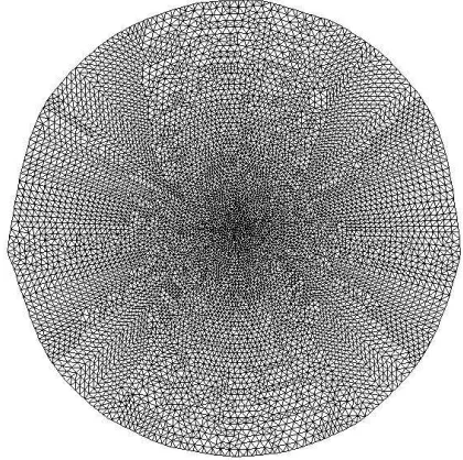
With the new method, the optimizer starts from the ini-tial shape (see Figure 1), which has about 3300 triangles, and the number of control points for this initial geom-etry is 22. After 37 optimization iterations it finds the optimum shape (see Figure 2), which has about 13,000 number of triangles because mesh refinement has been employed. This optimum shape has 40 control points be-cause the knot insertion algorithm has been incorporated. The value of the objective function at the optimum ge-ometry is−0.062333.
[image:3.595.319.529.79.288.2]The software used to solve the Poisson equation is that developed by Becker and Thompson [3].
Figure 1: Initial shape
Figure 2: optimum shape produced with the new method
The BFGS method used in the paper has been added the following enhancements: super-reduction, the geometry model, an algorithm to deal with self-intersection, and mesh refinement in order to deal with the constrained shape optimization problem. When the BFGS method is used, we starts from the same initial shape and with the same mesh. The optimizer takes 44 iterations to find the optimum shape. In terms of number of iterations, the new methods decreases the iteration counts by about 20%. The performance comparison of these two methods are shown in Figure 3.
Figure 3: Convergence performance comparison with BFGS method
[image:3.595.60.255.461.720.2] [image:3.595.320.534.496.605.2]Below is a table that reflects the influence of discretiza-tion error on the PDE soludiscretiza-tion:
number of nodes error in solution rate 814 0.0002161
3169 5.318e-05 4.06
Table 1: Discretization error analysis for the solution of Poisson’s equation
The above table shows that when the number of triangles is increased to about 4 times, then the discretization error will decrease to about 1/4, in agreement with theory.
4
Application for airfoil design
The purpose of this application is to find optimum shapes to minimize the drag of transonic airfoils while keeping the lift coefficient constant and keeping the maximum thickness of the airfoil constant. In this application, we follow Zhong and Qiao’s work [20] using the B-spline method to parameterize the geometry. The shape modifi-cations are parameterized by cubic B-splines with a nom-inal uniform knot set. The geometry of the airfoil is given by the following equation.
Y(Γ) =Y(Γini) + n
X
i=1
PiNi(X),
where Y(Γ), Y(Γini),represent the y coordinate of the
design geometry and initial geometry respectively,Piare
the control points of the B-spline, and Ni(X) are the
B-spline basis functions.
The transonic airfoil analysis code used in this pa-per is the NPUFOIL program, see [20]. The program is based on a combination of the full potential equation solver and the boundary layer flow analysis. The flow and the aerodynamic characteristics are computed via viscous/inviscid iteration. In this design case, the symmetric airfoil NACA0012 is chosen as the initial geometry. The lift coefficient CL = 0.5 , Mach number Ma = 0.77, and the Reynolds number Re = 6.5×10⁶
are kept unchanged. For comparison, both the new method and the EXTREM [15] method are used in this design case. For the new method, the geometry is first parameterized by 5 free control points, and finally it reaches the optimum solution which has 9 free control points and the drag is reduced from 0.0182 to 0.0070. The optimum solution of the control point is:
P1=−0.571028 P2=−0.70975 P3=−0.41511 P4= 0.13373 P5= 0.78084 P6= 1.3277 P7= 0.98959 P8= 0.56642 P9= 0.13606
The drag coefficient has been decreased by 62% (from 0.182 to 0.0070) for both methods, but the EXTREM method uses 408 function calls while the new method uses only 233. The CPU time per function call for these meth-ods, (CPU/FC) is nearly the same. The performance comparison table for the two methods is given below:
[image:4.595.315.540.308.456.2]Methods Cd iterations FC CPU/FC EXTREM 0.0070 N/A 408 0.22246 New Method 0.0070 20 233 0.22418 Table 2: Performance comparison of the new method and the EXTREM method
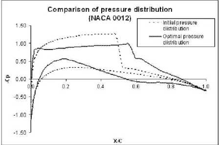
[image:4.595.315.538.530.706.2]Fig. 4 shows the comparison of pressure distribution in design case of NACA 0012, and Fig. 5 shows the com-parison of the drag coefficient for initial and optimal ge-ometry.
Figure 4: Initial and optimal pressure distribution for NACA 0012
5
Conclusions
In this paper, a new efficient method for shape opti-mization using B-spline shape functions combined with knot insertion algorithm and the super-reduced method is given. This method has good performance for both math-ematical problems and airfoil design applications. In the application to a Poisson’s equation problem, the new method uses only 37 iterations while the BFGS method uses 44 iterations.
In the airfoil design case, the drag coefficient has been reduced significantly, by about 62% with only 233 function calls, saving about 42% CPU time compared to the EXTREM method. Using this technique researchers will be able to accelerate their optimization as long as B-spline shape functions are used to parameterize the geometry.
In the future we will extend the range of applica-tion to include 3-dimensional problems.
References
[1] Anderson, W.K., Venkatakrishnan, V., “Aerody-namic design optimisation on unstructured grids with a continuous adjoint formulation,” AIAA Re-port97-0643, 1997.
[2] Anderson, W.K., Nielsen, E.J., “Sensitivity analysis for Navier-Stokes equations on unstructured meshes using complex variables,” AIAA Journal V39, N1, pp 56-63, 2001.
[3] Becker, D., Thompson, C.P., “A novel, parallel PDE solver for unstructured grids,” 5th Interna-tional Conference on Large-scale Scientific Compu-tation, 2005.
[4] Bischof, C., Carle, A., Gorliss, G., Griewank, A., Hovland,P., ADIFOR, “Generating derivative codes from FORTRAN programs”, Scientific Program-ming, V1, N1, pp 11-29,1992.
[5] Bischof,C., Roh,L., Mauer-Oats, A.J., ADIC, “An extensible automatic differentiation tool ANSI-C”,
Software Practice and Experience, V27, N12, pp 1427-1456, 1997.
[6] Borggaard, J., Burns, J., “A sensitivity equation ap-proach to shape optimisation in fluid flows”,ICASE ReportNo.94-8, 1994.
[7] Burkardt, J., Gunzburger, M., “Sensitivity dis-crepenancy for geometric parameters”,ASME CFD for Design and Optimisation, V232, pp 9-15, 1995. [8] Farin, G.E.,Curves and surfaces for CAGD: a
prac-tical guide5th edition, San Diego: Academic Press, 2002.
[9] Fletcher, R.,Practical methods of optimisation sec-ond edition, Wiley, 1987
[10] Hicks, R.M., Henne, P.A., “Wing design by numer-ical optimization”, AIAA 77-1247, AIAA Aircraft System and Technology Conference, Seattle, Wash., 1977.
[11] Hicks, R.M., Vanderplaats, G.N., “Application of numerical optimization to the design of supercriti-cal airfoils without drag-creep”,SAE paper 770440, 1977.
[12] Iollo, A., Kuruvila, G., Ta’asan, S., “Pseudo-time method for optimal shape design using the Euler equations”,ICASE ReportNo. 93-78, 1993.
[13] Jameson, A., “Aerodynamic design via control the-ory”,Journal of scientific computing, V3, N3, 1988. [14] Jameson, A., “Optimum aerodynamic design using CFD and control theory”, AIAA Paper 95-1729, 1995.
[15] Jacob, H.G., Rechnergestutzte optimierung statis-cher and dynamisstatis-cher system, Springer, Verlag, 1982.
[16] Lee, K.D., Eyi, S., “Transonic airfoil design by con-strained optimisation”, AIAA 91-3287, AIAA 9th Applied Aerodynamics Conference, Baltimore, MD, 1991.
[17] Lee, K.D., Eyi, S., “Transonic airfoil design by con-strained optimisation”,Journal of aircraft, V30, N6, 1993.
[18] Sherar, P.A., Thompson, C.P., Xu, B., Zhong, B., “A Novel Shape Optimization Method Using Knot Insertion Argorithm in B-Spline and Its Application to Transonic Airfoil Design”,Computer methods in Applied Mechanics and Engineering, [in preparation] 2007.
[19] Xie, L.,Gradient-based optimum aerodynamic design using adjoint-methods, PhD thesis of Virginia Poly-technic Institute and State University, 2002