Proceedings of the 2011 Conference on Empirical Methods in Natural Language Processing, pages 571–582,
Personalized Recommendation of User Comments via Factor Models
Deepak Agarwal Bee-Chung Chen Bo Pang Yahoo! Research
701 First Ave Sunnyvale, CA 94089
{dagarwal,beechun,bopang}@yahoo-inc.com
Abstract
In recent years, the amount of user-generated opinionated texts (e.g., reviews, user com-ments) continues to grow at a rapid speed: fea-tured news stories on a major event easily at-tract thousands of user comments on a popular online News service. How to consume subjec-tive information of this volume becomes an in-teresting and important research question. In contrast to previous work on review analysis that tried to filter or summarize information
for a genericaverageuser, we explore a
dif-ferent direction of enabling personalized rec-ommendation of such information.
For each user, our task is to rank the comments associated with a given article according to personalized user preference (i.e., whether the user is likely to like or dislike the comment). To this end, we propose a factor model that incorporates rater-comment and rater-author interactions simultaneously in a principled way. Our full model significantly outperforms strong baselines as well as related models that have been considered in previous work.
1 Introduction
Recent years have seen rapid growth in user-generated opinions online. Many of them are user reviews: a best-seller or a popular restaurant can get over 1000 reviews on top review sites like Ama-zon or Yelp. A large quantity of them also come in the form of user comments on blogs or news arti-cles. Most notably, during the short period of time for which a major event is active, news stories on one single event can easily attract over ten thousand
comments on a popular online news site like Yahoo! News. One question becomes immediate: how can we help people consume such gigantic amount of opinionated information?
One possibility is to take the summarization route. Briefly speaking (see Section 2 for a more detailed discussion), previous work has largely formulated review summarization as automatically or manually identify ratable aspects, and present overall senti-ment polarity for each aspect (Hu and Liu, 2004; Popescu and Etzioni, 2005; Snyder and Barzilay, 2007; Titov and McDonald, 2008). A related line of research looked into predicting helpfulness of re-views in the hope of promoting those with better quality, where helpfulness is usually defined as some function over the percentage of users who found the review to be helpful (Kim et al., 2006; Liu et al., 2007; Danescu-Niculescu-Mizil et al., 2009). In short, the focus of previous work has been on dis-tilling subjective information for anaverageuser.
new items.
Can we provide similar recommendation mech-anisms to help users consume large quantities of subjective information? Many commenting environ-ments allow users to mark “like” or “dislike” over existing comments (e.g., Yahoo! News comments, Facebook posts, or review sites that allow helpful-ness votes). Can we learn from users’ past prefer-ences, so that when a user is reading a new article, we have a system that automatically ranks its com-ments according to their likelihood of being liked by the user? This can be used directly to create person-alized presentation of comments (e.g., into a “like” column and a “dislike” column), as well as enabling down-stream applications such as personalized sum-marization.
Recommending textual information has recently attracted more attention. So far, the focus has been mainly on recommending news articles (Ahn et al., 2007; Das et al., 2007). Our task differs in several aspects. Intuitively, recommending news articles is largely about identifying the topics of interest to a given user, and it is conceivable that unigram repre-sentation of full-length articles can reasonably cap-ture that information. In our case, most comments for an article a user is reading are already of interest to that user topically. Which ones the user ends up liking may depend on several non-topical aspects of the text: whether the user agrees with the viewpoint expressed in the comment, whether the comment is convincing and well-written, etc. Previous work has shown that such analysis can be more difficult than topic-based analysis (Pang and Lee, 2008), and we have the additional challenge that comments are typ-ically much shorter than full-length articles. How-ever, the difficulty in analyzing the textual infor-mation in comments can be alleviated by additional contextual information such as author identities. If between a pair of users one consistently likes or dis-likes the other, then at least for the heavy users, this authorship information alone could be highly infor-mative. Indeed, previous work in collaborative filter-ing has usually found no additional gain from lever-aging content information when entity-level prefer-ence information is abundant.
In this paper, we present a principled way of uti-lizing multiple sources of information for the task of recommending user comments, which significantly
outperforms strong baseline methods, as well as pre-vious methods proposed for text recommendation. While using authorship information alone tends to provide stronger signal than using textual informa-tion alone, to our surprise, even for heavy users, adding textual information to the authorship infor-mation yields additional improvements.
2 Related Work
There are two main bodies of related work: our problem formulation is closer to collaborative filter-ing, while the nature of the text we are dealing with has more in common with opinion mining and sen-timent analysis.
Our approach is related to a large body of work in collaborative filtering. While a proper survey is not possible here, we describe some of the ap-proaches that are germane. Classical apap-proaches in collaborative filtering are based on item-item/user-user similarity, these are nearest-neighbor methods where the response for a user-item pair is predicted based on a local neighborhood mean (Sarwar et al., 2001; Wang et al., 2006). In general, neighbor-hoods are defined by measuring similarities between users/items through correlation measures like Pear-son, cosine similarities, etc. Better approaches to estimate similarities have also been proposed in Ko-ren (2010). However, modern methods based on matrix factorization have been shown to outperform nearest neighbor methods (Salakhutdinov and Mnih, 2008a,b; Bell et al., 2007). Generalizations of ma-trix factorization to include both features and past ratings have been proposed (Agarwal and Chen, 2009; Stern et al., 2009). The approach in this pa-per is an extension where in addition to interactions among users and items (comments in our case), we also consider the authorship information. Three-way interactions were recently studied for personalized tag recommendation (Rendle and Lars, 2010). Their model was based on the sum of two-way interac-tions, and was trained by using pairwise tag pref-erences for each (user, item) pair. However, no fea-tures were considered, which is an important consid-eration for us. We show using both text and author-ship provides the best performance.
years. For instance, Billsus and Pazanni (2007) de-scribes an approach to build user profile models for adaptive personalization in the context of mobile content access. Their approach is based on a hybrid model that combines content-based approaches with similarity methods used in recommender systems. This is further exemplified in the work by Ahn et al. (2007) where text processing techniques are used to build content profiles for users to recommend per-sonalized news. In our experiments, we show that such approaches are inferior to our method. A con-tent agnostic approach based on collaborative filter-ing techniques was proposed by Das et al. (2007); cold-start for new items/users was not their focus, but is important for our task — candidate comments for recommendation are often not in training data.
As discussed in Section 1, previous work in opin-ion mining and sentiment analysis has addressed the information consumption challenge via review sum-marization. Discussion of early work in that di-rection can be found in Pang and Lee (2008). In this line of work, opinions for each given aspect are usually summarized as the average sentiment po-larity associated with that aspect. Related to that, people have looked into predicting review helpful-ness given the textual information in reviews, where helpfulness is either defined as the percentage of users who have voted the review to be helpful (Kim et al., 2006), or labeled by annotators according to a set of criteria (Liu et al., 2007). Our goal dif-fers in that we look for personalized ranking (what a specific user might like) rather than generic qual-ity (what an average user might like). Subsequently, there has been work that tried to predict similarly defined helpfulness scores using meta-information over the reviewer. For instance, whether the au-thor has used his/her true name or where the user is from (Danescu-Niculescu-Mizil et al., 2009), as well as graph structure in the social network be-tween reviewers (Lu et al., 2010). In this work, we simply use author identity to provide more context to the short text; in future work, additional meta-information over users can easily be incorporated via our model.
As discussed in Section 1, whether a rater likes a comment or not may depend on whether they agree with the viewpoint expressed in the text and quality of the text. While previous work has not looked into
the reader-comments relationship, there has been re-lated work on identifying political orientations or viewpoints (Lin and Hauptmann, 2006; Lin et al., 2006; Mullen and Malouf, 2006, 2008; Laver et al., 2003); whether a piece of text expresses support or opposition in congressional debates (Thomas et al., 2006) or online debates (Somasundaran and Wiebe, 2009, 2010); as well as identifying contrastive re-lationship (Kawahara et al., 2010). Note that it is not trivial to use previous work along this line to di-rectly serve as sub-components in our setting. For instance, for work on identifying political orienta-tions or viewpoints, the training data consists of text with the desired labels. In our setting, our labels come in the form of whether users liked or disliked a previous comment. In the simplest case, we might have pair-wise constraints on whether two pieces of text have the same viewpoints (i.e., liked or dis-liked by the same rater), which would yield a dif-ferent learning problem akin to the metric learning problem; note, however, the complication that two pieces of text receiving different labels from a given user might not necessarily contain contrasting view-points. Consequently, rather than trying to reduce this problem to a set of known text classification tasks, we address this task via a collaborative filter-ing framework that incorporates textual features.
3 Method
3.1 Model
Notation:Letyijdenote the rating that useri, called
therater, gives to commentj. Since throughout, we use suffixito denote a rater and suffixjto denote a comment, we slightly abuse notation and letxi (of
dimensionpu) andxj(of dimensionpc) denote
fea-ture vectors of user i and comment j respectively. For example,xi can be the bag of words
represen-tation (a sparse vector) inferred through text anal-ysis on comments voted positively by user iin the past, andxj can be the bag of words representation
for commentj. We usea(j)to denote the author of
commentj, and useµijto denote the mean rating by
raterion commentj, i.e.,µij =E(yij). Of course it
is impossible to estimateµij empirically since each
useriusually rates a commentjat most once.
Model specification: We work in a generalized linear model framework (McCullagh and Nelder, 1989) that assumesµij (or some monotone function
hofµij) is an additive function of (1) the rater bias
αi of userisince some users may have a tendency
of rating comments more positively or negatively than others, (2) popularityβj of commentj, which
could reflect the quality of the comment in this set-ting, and (3) the author reputationγa(j)of usera(j) since comments by a reputed author may in general get more positive ratings. Thus, the overall bias is αi+βj+γa(j).
In addition to the bias, we include terms that capture interactions among entities (raters, authors, comments). Indeed, capturing such interactions is a non-trivial part of our modeling procedure. In our approach, we take recourse to factor models that have been widely used in collaborative filtering ap-plications in recent times. The basic idea is to at-tach latent factors to each rater, author and comment. These latent factors are finite dimensional Euclidean vectors that are unknown and estimated from the data. They provide a succinct representation of vari-ousaspectsthat are important to explain interaction among entities. In our case, we use the following factors — (a) user factor vi of dimension rv(≥ 1)
to model rater-author affinity, (b) user factorui and
comment factorcj of dimensionru(≥ 1)to model
rater-comment affinity. Intuitively, each could repre-sent viewpoints of users or comments along different
i index for raters j index for comments a(j) author of commentj
yij rating given by raterito commentj
µij mean rating given by raterito commentj xj feature vector of commentj
(e.g., textual features in commentj)
xi feature vector of useri
(e.g., comments voted positively by useri) bias terms:
αi rater bias of useri
βj popularity of commentj
(e.g., quality of the comment)
γa(j) reputation of the author of commentj interaction terms:
[image:4.612.311.552.70.305.2]vi user factor for rater-author affinity ui,cj factors for rater-comment affinity
Table 1: Table of Notations.
dimensions.
Affinity of rater i to comment j by author a(j)
is captured by (1) similarity between viewpoints of usersianda(j), measured byvi0va(j); and (2) simi-larity between the preferences of useriand the per-spectives reflected in commentj, measured byu0icj.
The overall interaction isv0iva(j)+u0icj.Then, the
mean ratingµij, or more preciselyh(µij), is
mod-eled as the sum of bias and interaction terms. Math-ematically, we assume:
yij ∼N(µij, σy2)or Bernoulli(µij)
h(µij) =αi+βj+γa(j)+v0iva(j)+u0icj
(1)
For numeric ratings, we use the Gaussian distri-bution denoted by N(mean,var); for binary rat-ings, we use the Bernoulli distribution. For Gaus-sian, h(µij) = µij, and for Bernoulli, we assume
h(µij) = log1−µijµij, which is the commonly used
logistic transformation.
Table 1 summarizes the notations for easy refer-ences. We denote the full model specified above as vv+uc since both user-user interaction vi0va(j) and
user-comment interaction u0icj are modeled at the
same time.
not work in our scenario since a large fraction of entities have small sample size. For instance, if a comment is rated only by one user and ru > 1,
the model is clearly overparametrized and the MLE of the comment factor would tend to learn idiosyn-crasies in the training data. Hence, it is imperative to impose constraints on the factors to obtain esti-mates that generalize well on unseen data. We work in a Bayesian framework where such constraints are imposed through prior distributions. The crucial is-sue is the selection of appropriate priors. In our sce-nario, we need priors that provide a good backoff
estimate when interacting entities have small sam-ple sizes. For instance, to estimate latent factors of a user with little data, we provide a backoff estimate that is obtained by pooling data across users with the same user features. We perform such a pooling through regression, the mathematical specification is given below.
αi ∼N(g0xi, σ2α), ui ∼N(Gxi, σu2),
βj ∼N(d0xj, σβ2), cj ∼N(Dxj, σ2c),
γa(j) ∼N(0, σ2γ), vi ∼N(0, σ2v),
where gpu×1 anddpc×1 are regression weight vec-tors, andGru×pu andDru×pc are regression weight matrices. These regression weights are learnt from data and provide the backoff estimate. Take the prior distribution of ui for example. We can rewrite the
prior as ui = Gxi +δi, whereδi ∼ N(0, σ2u).
If user ihas no rating in the training data, ui will
be predicted as the prior mean (backoff)Gxi, a
lin-ear projection from the feature vector xi through
matrix Glearnt from data. This projection can be thought of as a multivariate linear regression prob-lem with weight matrix G, one weight vector per dimension of ui. However, if userihas many
rat-ings in the training data, we will precisely estimate the per-userresidualδithat is not captured by the
re-gressionGxi. For sample sizes in between these two
extremes, the per user residual estimate is “shrunk” toward zero — amount of shrinkage depends on the sample size, past user ratings, variability in ratings on comments rated by the user, and the value of vari-ance componentsσ2·s.
3.2 Special Cases of Our Model
Our full model (vv+uc) includes several existing models explored in collaborative filtering and social
networks as special cases.
The matrix factorization model: This model as-sumes the mean rating of user ion itemj is given by h(µij) = αi + βj + u0icj, and the mean of
the prior distributions onαi, βj,ui,cj are zero, i.e.,
g = d = G = D = 0.Recent work clearly illus-trates that this method obtains better predictive accu-racy than classical collaborative filtering techniques based on item-item similarity (Bell et al. (2007)).
The uc model: This is also a matrix factorization model but with priors based on regressions (i.e., non-zero g, d, G, D). It provides a mechanism to deal with both cold and warm-start scenarios in rec-ommender applications (Agarwal and Chen (2009)).
Thevvmodel: This model assumesh(µij) = αi+
γa(j)+vi0va(j).It was first proposed by Hoff (2005) to model interactions in social networks. The model was fitted to small datasets (at most a few hundred nodes) and the goal was to test certain hypotheses on social behavior, out-of-sample prediction was not considered.
The low-rank bilinear regression model: Here, h(µij) = g0xi +d0xj +x0iG0Dxj. This is a
re-gression model purely based on features with no per-user or per-comment latent factors. In a more gen-eral form,x0iG0Dxjcan be written asx0iAxj, where
Apu×pcis the matrix of regression weights (Chu and Park, 2009). However, sincexiandxj are typically
high dimensional,Acan be a large matrix that needs to be learnt from data. To reduce dimensionality, one can decomposeAasA = G0D, where the number of rows inDandGare small. Thus, instead of learn-ingA, we learn a low-rank approximation ofA. This ensures scalability and provides an attractive method to avoid over-fitting.
3.3 Model Fitting
Model fitting for our model is based on the expectation-maximization (EM) algorithm (Demp-ster et al., 1977). For ease of exposition and space constraints, we only provide a sketch of the algo-rithm for the Gaussian case, the logistic model can be fitted along the same lines by using a variational approximation (see Agarwal and Chen (2009)).
Let Y = {yij} denote the set of the observed
data that gets augmented with the latent factors
Θ = {ui,vi,cj} to obtain the “complete” data.
The goal of the EM algorithm is to find the param-eterη = (g, d, G, D, σ2
α, σβ2, σu2, σv2, σy2)that
maxi-mizes the “incomplete” data likelihoodPr(Y|η) =
R
Pr(Y,Θ|η)dΘthat is obtained after
marginaliza-tion (taking expectamarginaliza-tion) over the distribumarginaliza-tion ofΘ.
Since such marginalization is not available in closed form for our model, we use the EM algorithm. EM algorithm: The complete data log-likelihood l(η;Y,Θ) for the full model in the Gaussian case
(whereh(µij) =µij) is given byl(η;Y,Θ) =
−12
P
ij (yij−µij)2/σy2+ logσy2
−1 2
P
i (αi−g0xi)2/σ2α+ logσ2α
−12Pj
(βj−d0xj)2/σβ2 + logσβ2
−12
P
i kui−Gxik2/σu2+rulogσ2u
−12
P
j kcj−Dxjk2/σc2+rulogσc2
,
−1 2
P
i v0ivi/σ2v+rvlogσv2+γi2/σ2γ+ logσγ2
,
whereruis the dimension of factorsui andcj, and
rv is the dimension ofvi. Letη(t) denote the
esti-mated parameter setting at thetthiteration. The EM algorithm iterates through the following two steps until convergence.
• E-step:Computeft(η) =EΘ[l(η;Y,Θ)|η(t)] as a function ofη, where the expectation is taken over the posterior distribution of (Θ|η(t),Y).
Note that hereηis the input variable of function
ft, butη(t) consists of known quantities
(deter-mined in the previous iteration).
• M-step: Find theηthat maximizes the
expecta-tion computed in the E-step.
η(t+1) = arg max
η ft(η)
Since the expectation in the E-step is not available in a closed form, we use a Gibbs sampler to compute the Monte Carlo expectation (Booth and Hobert, 1999). The Gibbs sampler repeats the following procedure L times. It samples αi, γi, βj, ui, vj,
andcj sequentially one at a time by sampling from
the corresponding full conditional distributions. The full conditional distributions are all Gaussian, hence they are easy to sample. Once a Monte Carlo ex-pectation is calculated from the samples, an updated
estimate ofη is obtained in the M-step. The
opti-mization of variance componentsσ2
·s in the M-step
is available in closed form, the regression param-eters are estimated through off-the-shelf linear re-gression routines. We note that the posterior distri-bution of latent factors for knownηis multi-modal,
we have found the Monte Carlo based EM method to outperform other optimization methods like gradient descent in terms of predictive accuracy.
4 Experiments 4.1 Data
We obtained comment rating data between March and May, 2010 from Yahoo! News, with all user IDs anonymized. On this site, users can post comments on news article pages and rate the comments made by others through up (positive) or thumb-down (negative) votes. Clearly, for articles with very few comments, there is no need to recommend com-ments. Also, we do not expect deep personalized recommendations for users who have rated very few comments in the past. To focus on instances of in-terest to us, we restricted ourselves to a subset of the rating data associated with relatively heavy raters. In particular, we formed the experimental dataset by randomly selecting 9,003 raters who provided at least 200 ratings (of which at least 10 were posi-tive and 10 were negaposi-tive), 189,291 authors who re-ceived at least 20 ratings, and 5,088 news articles that received at least 40 comments in the raw dataset during the three-month period. Note that the per en-tity sample size in the experimental dataset can be smaller than the thresholds specified above. For in-stance, a rater with more than 200 ratings in the raw dataset can have fewer than 200 in the experimental dataset due to the removal of certain authors or news articles. (See Figure 2 for a distribution of users with different activity levels.) In total, we have 4,440,222 ratings on 1,197,098 comments.
this training-test split ensures that performance on the test data best simulates our application scenar-ios. It also creates a completely cold-start situation for comments — no comment in the test set has any past rating in the training set.
4.2 Experimental Setup
Features: All comments were tokenized, lower-cased, with stopwords and punctuations removed. We limited the vocabulary to the 10K most frequent tokens in all comments associated with the training articles. (See Section 4.3.3 for a discussion on the effect of the vocabulary size.) For a given comment j,xj is its bag of words representation,L2 normal-ized. For term weighting, we experimented with both presence value and tf-idf weighting. The latter gives slight better performance. Rater feature vector
xi is created by summing over the feature vectors
of all comments rated positively by rateri, which is thenL2 normalized.
Methods: We compare the following methods based on our model: The full modelvv+uc, as well as the three main special cases, vv, uc, and bilin-ear, as defined in Section 3. The dimensions ofvi, ui and cj (i.e., rv and ru), and the rank of
bilin-earare selected to obtain the best AUC on the tun-ing set. In our experiments, rv = 2, ru = 3 and
rank ofbilinearis 3. In addition, we also evaluate the following baseline methods that predict per-user preferences in isolation, primarily based on textual information.
• Cosine similarity (cos): x0ixj. This is simply
based on how similar a new commentjis to the comments raterihas liked in the past.
• Per-user SVM (svm):For each rater, train a sup-port vector machine (SVM) classifier using only comments (xj) rated by that user.
• Per-user Naive Bayes (nb):For each rater, train a Naive Bayes classifier using only comments (xj) rated by that user.1
Note that SVMs typically yield the best performance on text classification tasks; a Naive Bayes classifier 1As we mentioned in Section 4.1, not all users have training data of both classes in the experimental dataset. Forsvmand nb, we use the following backoff: for users with training data from onlyci, we predictci; for users with no training data at all, we predict the majority class, in this case, the positive class.
can be more robust over shorter text spans common in user comments given the high variance. For fair comparisons, for the three baseline methods, we use a simple way of utilizing author information: the feature space is augmented with author IDs and each
xjis augmented witha(j)2. In Section 4.3, we only
report results using the augmented feature vectors since they yield better performance (though the dif-ference is fairly small).
Performance metrics: We use two types of met-rics to measure the performance of a method: (1) A global metric based on Receiver Operating Char-acteristic (ROC) and (2) Precision at rankk(P@k). The former measures the overall correlation of pre-dicted scores for a method with the observed rat-ings in the test set, while the latter measures the performance of a hypothetical top-k recommenda-tion scenario using the method. To summarize an ROC curve into a single number, we use the Area Under the ROC Curve (AUC). Since random guess yields AUC score of 0.5, regardless of the class dis-tribution, using this measure makes it convenient for us to compare the performance over different sub-sets of the data (where class distributions could be different). The P@k of a method is computed as follows: (1) For each rater, rank comments that the rater rated in the test set according to the scores pre-dicted by the method, and compute the precision at rankk for that rater; and then (2) average the per-rater precision numbers over all per-raters. To report P@k, fork= 5,10,20, we only use raters who have at least 50 ratings in the test set. Statistical signif-icance based on a two-sample t-test across raters is also reported.
4.3 Results
4.3.1 Main comparisons
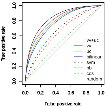
We first show the ROC curves of different meth-ods on the test set in Figure 1, and the AUCs and precisions in Table 2. Results from significance tests are in Table 3.
False positive rate
T
rue positiv
e r
ate
0.0 0.2 0.4 0.6 0.8 1.0
0.0 0.2 0.4 0.6 0.8 1.0
False positive rate
T
rue positiv
e r
ate
0.0 0.2 0.4 0.6 0.8 1.0
0.0 0.2 0.4 0.6 0.8 1.0
False positive rate
T
rue positiv
e r
ate
0.0 0.2 0.4 0.6 0.8 1.0
0.0 0.2 0.4 0.6 0.8 1.0
False positive rate
T
rue positiv
e r
ate
0.0 0.2 0.4 0.6 0.8 1.0
0.0 0.2 0.4 0.6 0.8 1.0
False positive rate
T
rue positiv
e r
ate
0.0 0.2 0.4 0.6 0.8 1.0
0.0 0.2 0.4 0.6 0.8 1.0
False positive rate
T
rue positiv
e r
ate
0.0 0.2 0.4 0.6 0.8 1.0
0.0 0.2 0.4 0.6 0.8 1.0
False positive rate
T
rue positiv
e r
ate
0.0 0.2 0.4 0.6 0.8 1.0
[image:8.612.319.535.70.182.2]0.0 0.2 0.4 0.6 0.8 1.0 vv+uc vv uc bilinear svm nb cos random
Figure 1: ROC curves of different models
Method AUC P@5 P@10 P@20
vv+uc 0.8360 0.9152 0.9079 0.8942 vv 0.8090 0.8810 0.8807 0.8727 uc 0.7857 0.9046 0.8921 0.8694 bilinear 0.7701 0.9028 0.8894 0.8668 svm 0.6768 0.7814 0.7678 0.7497 nb 0.6465 0.7660 0.7486 0.7309 cos 0.5382 0.6834 0.6813 0.6754
Table 2: AUCs and precisions of different models.
rather than in isolation. Next,ucoutperforms bilin-ear(significantly in AUC, P@10 and P@20), show-ing per-user and per-comment latent factors help. Note that vv outperforms uc in ROC, AUC and P@20, but is worse thanucin P@5 and P@10; we will take a closer look at this later. Finally, the full modelvv+ucsignificantly outperforms bothvvand uc, achieving 0.83 in AUC, and close to 90% in pre-cision at rank 20.
4.3.2 Break-down by user activity level
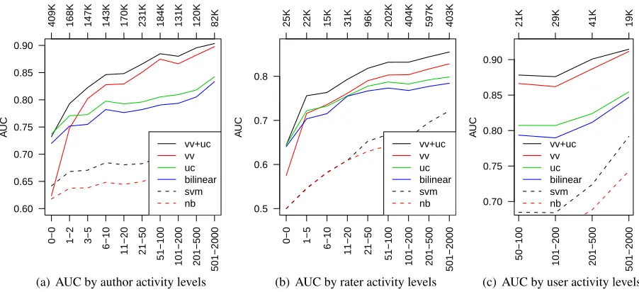
Next, we investigate model performance in differ-ent subsets of the test set. For succinctness, we use AUC as our performance metric. In Figure 2(a), we breakdown model performance by different author activity levels. In Figure 2(b), we breakdown model performance by different voter activity levels. We also generated similar plots with the y-axis replaced by P@5, P@10 and P@20, and observed the same trend except thatvvstarts to outperformucat differ-ent user activity thresholds for differdiffer-ent metrics.
Comparison Metrics p-value vv+uc>vv All <10−7 vv+uc>uc All <10−20
uc>bilinear All except P@5 <0.006
bilinear>svm All <10−20 vv>svm All <10−20
svm>nb All <10−8
nb>cos All <10−20
Table 3: Paired t-test results. Note thatucis better than
bilinearin P@5, but not significant. The orders ofuc
andvvare not consistent across different metrics.
Not surprisingly,vvperforms poorly for raters or authors with no ratings observed in the training data. However, once we have a small amount of ratings, it starts to outperformuc, even though intuitively, the textual information in the comment should be more informative than the authorship information alone. Using paired t-tests with significance level 0.05, we report whenvvstarts to significantly outperformuc in the following table, which is interpreted as fol-lows —vvis not significantly worse thanucin met-ric M if the author of a test comment received at leastNeq ratings in the training set, andvv signifi-cantly outperformsucin metricM if the author re-ceived at leastNgtratings in the training set.
MetricM P@5 P@10 P@20 AUC
# RatingsNeq 50 5 5 5
Ngt 1000 50 5 5
Recall that our training/test split is by article. Since we have never observed a rater’s preference over the test articles before, it is rather surprising that author information alone can yield 0.8 in AUC score, even for very light authors who have received between 3 and 5 votes in total in the training data. This suggests that users’ viewpoints are quite consistent: a large portion of the ratings can be adequately explained by the pair of user identities. One interesting obser-vation is that the number of ratings required forvvto outperformucin P@5 is quite high. This suggests that to obtain high precision at the top of a recom-mended list, comment features are important.
[image:8.612.84.266.71.255.2]signifi-0.60 0.65 0.70 0.75 0.80 0.85 0.90
A
UC
0−0 1−2 3−5
6−10
11−20 21−50
51−100 101−200 201−500
501−2000
409K 168K 147K 143K 170K 231K 184K 131K 120K 82K
vv+uc vv uc bilinear svm nb
(a) AUC by author activity levels
0.5 0.6 0.7 0.8
A
UC
0−0 1−5
6−10
11−20 21−50
51−100 101−200 201−500
501−2000
25K 22K 15K 31K 96K 202K 404K 597K 403K
vv+uc vv uc bilinear svm nb
(b) AUC by rater activity levels
0.70 0.75 0.80 0.85 0.90
A
UC
50−100 101−200 201−500
501−2000
21K 29K 41K 19K
vv+uc vv uc bilinear svm nb
[image:9.612.73.524.79.285.2](c) AUC by user activity levels
Figure 2: AUC of different models as a function of the activity level of authors or raters. The x-axis (bottom) has the
formm-n, meaning the subset of the test data in which the number of ratings that each author received (as in (a)) or
each rater gave (as in (b)) in the training set is betweenmandn. In (c), we select both authors and raters based on the
m-ncriterion. The x-axis (top) denotes the number of ratings in the subset
cance level 0.05,vv+ucsignificantly outperformsvv in all metrics if the author received < 500 ratings
in the training set. Except for the very heavy au-thors, even for cases where both raters and authors are heavy users (Figure 2(c)), adding the comment feature information still yields additional improve-ment over the already impressive performance of us-ingvvalone. In spite of the simple representation we adopted for the textual information, the full model is still capable of accounting for part of the residual errors fromvvmodel (that uses authorship informa-tion alone) by using comment features — what was actually written does matter.
Finally, if we breakdown the comparison be-tweenvv+uc anduc for different user activity lev-els, vv+uc significantly outperformsuc (with level 0.05) in all metrics if the author received at least 5 ratings in the training set.
4.3.3 Analysis of textual features
Recall that we limited the vocabulary size to the 10K most frequent terms for efficiency reasons. Is this limitation likely to affect our model perfor-mance significantly? We examined the effect of dif-ferent numbers of features. In the following table, #features = n means that both xi andxj are bags
of n words3. Since the vv model does not utilize rater or comment features, we examine AUC of the ucmodel.
#features 1K 3K 5K 10K
AUC 0.7713 0.7855 0.7872 0.7876
As can be seen, the performance improvement is in the 4th decimal place when we increase from 5K features to 10K features. Thus, we do not further increase the number of features in our experiments.
Note that our full model does not require rater fea-tures and comment feafea-tures to be in the same feature space. Each is projected into the hidden “viewpoint” space, viaGandD, separately. For simplicity and easy comparison to other methods, we used all com-ments liked by a rater in the past to build the feature vector of the rater. But since the full model already has information of the textual content of comments from the comment features, and which comments were liked by the users from the ratings, rater fea-tures constructed this way do not provide any new information. Indeed, if we modelui ∼ N(1, σu2),
instead ofui ∼ N(Gxi, σu2), this omission of xi
does not hurt the performance of the model. In fu-ture work, other meta-information about the rater
can easily be incorporated intoxito enrich rater
rep-resentation.
Recall that comment featuresxjwere projected to
comment factorscj viaD. We envisioned that the
comment factors could be representing viewpoints. Does our model conform to this intuition? Let’s con-sider the simplest case, where we restrictui andcj
to be one-dimensional vectors. In this case, each can be represented by scalars ui and cj. If ui and cj
are of the same sign, then the rater is likely to like the comment. Words assigned high positive weights or low negative weights viaDwill have significant contributions to the overall sign ofcj. Now if we
ex-amine such words, will we see any meaningful dif-ferences in the underlying viewpoints of these two groups of words?
To address this question qualitatively, we manu-ally sampled words with heavy weights, focusing on politics-related ones (so that viewpoints are likely to be polarized and easier to interpret). At one ex-treme, we observe words likerepukes, repugs, which seemed to be derogatory mentions of Republica-tions, and likely to represent an anti-Republication point of view. At the other end, we observe terms like libtards, nobama, obummer. While terms like
nobama may appear to be typos at first sight, a quick search online reveals that these are at least intentional typos expressing anti-Obama sentiments, which clearly represents an opposite underlying per-spective from terms likerepukes.
These examples also illustrate the importance to learn directly from the data of interest to us. Such indicative words would never have appeared in more formal writings. While we do not have direct labels for perspectives, our model seems to be capturing the underlying perspectives (as much as a unigram-based model could) by learning from user preference labels across different users. This allows us to learn the text features most relevant to our dataset, which is particularly important given the time-sensitive and ever-evolving nature of news-related comments.
5 Conclusions
In this paper, we promote personalized recommen-dation as a novel way of helping users to consume large quantities of subjective information. We pro-pose using a principled way of incorporating both
rater-comment and rater-author interactions simul-taneously. Our full model significantly outperforms strong baseline methods, as well as previous meth-ods proposed for text recommendation. In particu-lar, learning weights over textual features across all users outperforms learning for each user individu-ally, which holds true even for heavy raters. Further-more, while using authorship information alone pro-vides stronger signal than using textual information alone, to our surprise, even for heavy users, adding textual information yields additional improvements. It is difficult to comprehensively capture user affinity to comments using a finite number of rat-ings observed during a certain time interval. News and comments on news articles are dynamic in na-ture, novel aspects may emerge over time. To cap-ture such dynamic behavior, comment factors have to be allowed to evolve over time and such an evolu-tion would also necessitate the re-estimaevolu-tion of user factors. Incorporating such temporal dynamics into our modeling framework is a challenging research problem and requires significant elaboration of our current approach.
Acknowledgments
We thank the anonymous reviewers for useful sug-gestions.
References
D. Agarwal and B.C. Chen. Regression-based latent factor models. In Proceedings of the 15th ACM SIGKDD international conference on Knowledge discovery and data mining, pages 19–28. ACM, 2009.
Jae-Wook Ahn, Peter Brusilovsky, Jonathan Grady, Daqing He, and Sue Y. Syn. Open user profiles for adaptive news systems: help or harm? In Pro-ceedings of the 16th international conference on World Wide Web (WWW), 2007.
Robert Bell, Yehuda Koren, and Chris Volinsky. Modeling relationships at multiple scales to im-prove accuracy of large recommender systems. In
KDD, 2007.
D. Billsus and M. Pazanni. Adaptive news access. Springer, Berlin, 2007.
monte carlo EM algorithm. J.R.Statist. Soc. B, 1999.
Wei Chu and Seung T. Park. Personalized recom-mendation on dynamic content using predictive bilinear models. InProceedings of the 18th inter-national conference on World Wide Web (WWW), 2009.
Cristian Danescu-Niculescu-Mizil, Gueorgi Kossinets, Jon Kleinberg, and Lillian Lee. How opinions are received by online communi-ties: A case study on Amazon.com helpfulness votes. InProceedings of WWW, pages 141–150, 2009.
Abhinandan S. Das, Mayur Datar, Ashutosh Garg, and Shyam Rajaram. Google news personaliza-tion: scalable online collaborative filtering. In
Proceedings of the 16th international conference on World Wide Web (WWW), 2007.
A. P. Dempster, N. M. Laird, and D. B. Rubin. Max-imum likelihood from incomplete data via the EM algorithm. Journal of the Royal Statistical Soci-ety, Series B, 39:1–38, 1977.
Peter D. Hoff. Bilinear mixed-effects models for dyadic data. Journal of the American Statistical Association, 100(469):286–295, 2005.
Minqing Hu and Bing Liu. Mining and summa-rizing customer reviews. In Proceedings of the ACM SIGKDD Conference on Knowledge Dis-covery and Data Mining (KDD), pages 168–177, 2004.
Daisuke Kawahara, Kentaro Inui, and Sadao Kuro-hashi. Identifying contradictory and contrastive relations between statements to outline web infor-mation on a given topic. In Proceedings of the 23rd International Conference on Computational Linguistics (COLING): Posters, 2010.
Soo-Min Kim, Patrick Pantel, Tim Chklovski, and Marco Pennacchiotti. Automatically assessing re-view helpfulness. In Proceedings of the Confer-ence on Empirical Methods in Natural Language Processing (EMNLP), pages 423–430, Sydney, Australia, July 2006. Association for Computa-tional Linguistics.
Y. Koren. Factor in the neighbors: Scalable and ac-curate collaborative filtering. ACM Transactions
on Knowledge Discovery from Data (TKDD), 4 (1):1–24, 2010. ISSN 1556-4681.
Michael Laver, Kenneth Benoit, and John Garry. Ex-tracting policy positions from political texts using words as data.American Political Science Review, 97(2):311–331, 2003.
Wei-Hao Lin and Alexander Hauptmann. Are these documents written from different perspectives? A test of different perspectives based on sta tisti-cal distribution divergence. InProceedings of the International Conference on Computational Lin-guistics (COLING)/Proceedings of the Associa-tion for ComputaAssocia-tional Linguistics (ACL), pages 1057–1064, Sydney, Australia, July 2006. Asso-ciation for Computational Linguistics.
Wei-Hao Lin, Theresa Wilson, Janyce Wiebe, and Alexander Hauptmann. Which side are you on? identifying perspectives at the document and sen-tence levels. InProceedings of the Conference on Natural Language Learning (CoNLL), 2006. Jingjing Liu, Yunbo Cao, Chin-Yew Lin, Yalou
Huang, and Ming Zhou. Low-quality product review detection in opinion summarization. In
Proceedings of the Joint Conference on Empir-ical Methods in Natural Language Processing and Computational Natural Language Learning (EMNLP-CoNLL), pages 334–342, 2007. Poster paper.
Yue Lu, Panayiotis Tsaparas, Alexandros Ntoulas, and Livia Polanyi. Exploiting social context for review quality prediction. InProceedings of the 19th International World Wide Web Conference (WWW), 2010.
P. McCullagh and J. A. Nelder. Generalized Linear Models. Chapman & Hall/CRC, 1989.
Tony Mullen and Robert Malouf. A preliminary in-vestigation into sentiment analysis of informal po-litical discourse. InAAAI Symposium on Compu-tational Approaches to Analysing Weblogs (AAAI-CAAW), pages 159–162, 2006.
Tony Mullen and Robert Malouf. Taking sides: User classification for informal online political discourse. Internet Research, 18:177–190, 2008. Bo Pang and Lillian Lee. Opinion mining and
Ana-Maria Popescu and Oren Etzioni. Extracting product features and opinions from reviews. In
Proceedings of the Human Language Technol-ogy Conference and the Conference on Empir-ical Methods in Natural Language Pro cessing (HLT/EMNLP), 2005.
Steffen Rendle and Schmidt-Thie Lars. Pairwise interaction tensor factorization for personalized tag recommendation. InProceedings of the third ACM international conference on Web search and
data mining, WSDM ’10, pages 81–90, New
York, NY, USA, 2010. ACM.
R. Salakhutdinov and A. Mnih. Bayesian proba-bilistic matrix factorization using Markov chain Monte Carlo. In Proceedings of the 25th inter-national conference on Machine learning, pages 880–887. ACM, 2008a.
R. Salakhutdinov and A. Mnih. Probabilistic ma-trix factorization.Advances in neural information processing systems, 20:1257–1264, 2008b. Badrul Sarwar, George Karypis, Joseph Konstan,
and John Reidl. Item-based collaborative filter-ing recommendation algorithms. In WWW ’01: Proceedings of the 10th international conference on World Wide Web, pages 285–295. ACM, 2001. Benjamin Snyder and Regina Barzilay. Multiple as-pect ranking using the Good Grief algorithm. In
Proceedings of the Joint Human Language Tech-nology/North American Chapter of the ACL Con-ference (HLT- NAACL), pages 300–307, 2007. Swapna Somasundaran and Janyce Wiebe.
Recog-nizing stances in online debates. InProceedings
of the Joint Conference of the 47th Annual Meet-ing of the ACL and the 4th International Joint Conference on Natural Language Processing of the AFNLP, 2009.
Swapna Somasundaran and Janyce Wiebe. Recog-nizing stances in ideological on-line debates. In
Proceedings of the NAACL HLT 2010 Workshop on Computational Approaches to Analysis and Generation of Emotion in Text, 2010.
David H. Stern, Ralf Herbrich, and Thore Grae-pel. Matchbox: large scale online bayesian rec-ommendations. InProceedings of the 18th inter-national conference on World Wide Web (WWW), 2009.
Matt Thomas, Bo Pang, and Lillian Lee. Get out the vote: Determining support or opposition from Congressional floor-debate transcripts. In Pro-ceedings of the Conference on Empirical Methods in Natural Language Processing (EMNLP), pages 327–335, 2006.
Ivan Titov and Ryan McDonald. A joint model of text and aspect ratings for sentiment summariza-tion. InProceedings of the Association for Com-putational Linguistics (ACL), 2008.