Multi Timescale Long Short Term Memory Neural Network for Modelling Sentences and Documents

Multi-Timescale Long Short-Term Memory Neural Network

for Modelling Sentences and Documents

Pengfei Liu, Xipeng Qiu∗_{, Xinchi Chen, Shiyu Wu, Xuanjing Huang} Shanghai Key Laboratory of Intelligent Information Processing, Fudan University

School of Computer Science, Fudan University 825 Zhangheng Road, Shanghai, China

{pfliu14,xpqiu,xinchichen13,syu13,xjhuang}@fudan.edu.cn

Abstract

Neural network based methods have ob-tained great progress on a variety of nat-ural language processing tasks. However, it is still a challenge task to model long texts, such as sentences and documents. In this paper, we propose a multi-timescale long short-term memory (MT-LSTM) neu-ral network to model long texts. MT-LSTM partitions the hidden states of the standard LSTM into several groups. Each group is activated at different time peri-ods. Thus, MT-LSTM can model very long documents as well as short sentences. Experiments on four benchmark datasets show that our model outperforms the other neural models in text classification task.

1 Introduction

Distributed representations of words have been widely used in many natural language process-ing (NLP) tasks (Collobert et al., 2011; Turian et al., 2010; Mikolov et al., 2013b; Bengio et al., 2003). Following this success, it is rising a sub-stantial interest to learn the distributed represen-tations of the continuous words, such as phrases, sentences, paragraphs and documents (Mitchell and Lapata, 2010; Socher et al., 2013; Mikolov et al., 2013b; Le and Mikolov, 2014; Kalchbren-ner et al., 2014). The primary role of these mod-els is to represent the variable-length sentence or document as a fixed-length vector. A good rep-resentation of the variable-length text should fully capture the semantics of natural language.

Recently, the long short-term memory neural network (LSTM) (Hochreiter and Schmidhuber, 1997) has been applied successfully in many NLP tasks, such as spoken language understanding (Yao et al., 2014), sequence labeling (Chen et al.,

∗_{Corresponding author}

2015) and machine translation (Sutskever et al., 2014). LSTM is an extension of the recurrent neu-ral network (RNN) (Elman, 1990), which can cap-ture the long-term and short-term dependencies and is very suitable to model the variable-length texts. Besides, LSTM is also sensitive to word order and does not rely on the external syntactic structure as recursive neural network (Socher et al., 2013). However, when modeling long texts, such as documents, LSTM need to keep the useful features for a quite long period of time. The long-term dependencies need to be transmitted one-by-one along the sequence. Some important features could be lost in transmission process. Besides, the error signal is also back-propagated one-by-one through multiple time steps in the training phase with back-propagation through time (BPTT) (Werbos, 1990) algorithm. The learning efficiency could also be decreased for the long texts. For ex-ample, if a valuable feature occurs at the begin of a long document, we need to back-propagate the error through the whole document.

In this paper, we propose a multi-timescale long short-term memory (MT-LSTM) to capture the valuable information with different timescales. In-spired by the works of (El Hihi and Bengio, 1995) and (Koutnik et al., 2014), we partition the hidden states of the standard LSTM into several groups. Each group is activated and updated at different time periods. The fast-speed groups keep the short-term memories, while the slow-speed groups keep the long-term memories. We evaluate our model on four benchmark datasets of text classifi-cation. Experimental results show that our model can not only handle short texts, but can model long texts.

Our contributions can be summarized as fol-lows.

• With the multiple different timescale memo-ries, MT-LSTM easily carries the crucial in-formation over a long distance. MT-LSTM

can well model both short and long texts.

• MT-LSTM has faster convergence speed than the standard LSTM since the error signal can be back-propagated through multiple timescales in the training phase.

2 Neural Models for Sentences and Documents

The primary role of the neural models is to repre-sent the variable-length repre-sentence or document as a fixed-length vector. These models generally con-sist of a projection layer that maps words, sub-word units or n-grams to vector representations (often trained beforehand with unsupervised meth-ods), and then combine them with the different architectures of neural networks. Most of these models for distributed representations of sentences or documents can be classified into four cate-gories.

Bag-of-words models A simple and intuitive method is the Neural Bag-of-Words (NBOW) model, in which the representation of sentences or documents can be generated by averaging con-stituent word representations. However, the main drawback of NBOW is that the word order is lost. Although NBOW is effective for general docu-ment classification, it is not suitable for short sen-tences.

Sequence models Sequence models construct the representation of sentences or documents based on the recurrent neural network (RNN) (Mikolov et al., 2010) or the gated versions of RNN (Sutskever et al., 2014; Chung et al., 2014). Sequence models are sensitive to word order, but they have a bias towards the latest input words. This gives the RNN excellent performance at lan-guage modelling, but it is suboptimal for modeling the whole sentence, especially for the long texts. Le and Mikolov (2014) proposed a Paragraph Vec-tor (PV) to learn continuous distributed vecVec-tor rep-resentations for pieces of texts, which can be re-garded as a long-term memory of sentences as op-posed to the short-memory in RNN.

Topological models Topological models com-pose the sentence representation following a given topological structure over the words (Socher et al., 2011a; Socher et al., 2012; Socher et al., 2013). Recursive neural network (RecNN) adopts

a more general structure to encode sentence (Pol-lack, 1990; Socher et al., 2013). At every node in the tree the contexts at the left and right children of the node are combined by a classical layer. The weights of the layer are shared across all nodes in the tree. The layer computed at the top node gives a representation for the sentence. However, RecNN depends on external constituency parse trees provided by an external topological structure, such as parse tree.

Convolutional models Convolutional neural network (CNN) is also used to model sentences (Collobert et al., 2011; Kalchbrenner et al., 2014; Hu et al., 2014). It takes as input the embeddings of words in the sentence aligned sequentially, and summarizes the meaning of a sentence through layers of convolution and pooling, until reaching a fixed length vectorial representation in the final layer. CNN can main-tain the word order information and learn more abstract characteristics.

3 Long Short-Term Memory Networks A recurrent neural network (RNN) (Elman, 1990) is able to process a sequence of arbitrary length by recursively applying a transition function to its in-ternal hidden state vectorhtof the input sequence.

The activation of the hidden statehtat time-stept

is computed as a function f of the current input symbolxtand the previous hidden stateht−1

ht=

{

0 t= 0

f(ht−1,xt) otherwise (1)

It is common to use the state-to-state transition functionf as the composition of an element-wise nonlinearity with an affine transformation of both

xtandht−1.

Traditionally, a simple strategy for modeling se-quence is to map the input sese-quence to a fixed-sized vector using one RNN, and then to feed the vector to a softmax layer for classification or other tasks (Sutskever et al., 2014; Cho et al., 2014).

Figure 1: A LSTM unit. The dashed line is the recurrent connection, and the solid link is the con-nection at the current time.

Long short-term memory network (LSTM) was proposed by (Hochreiter and Schmidhuber, 1997) to specifically address this issue of learning long-term dependencies. The LSTM maintains a sepa-rate memory cell inside it that updates and exposes its content only when deemed necessary. A num-ber of minor modifications to the standard LSTM unit have been made. While there are numerous LSTM variants, here we describe the implementa-tion used by Graves (2013).

We define the LSTM units at each time stept

to be a collection of vectors inRd_{: aninput gate} it, aforget gate ft, an output gate ot, a memory cellct and a hidden state ht. dis the number of

the LSTM units. The entries of the gating vectors

it, ft and ot are in [0,1]. The LSTM transition equations are the following:

it=σ(Wixt+Uiht−1+Vict−1) (2)

ft=σ(Wfxt+Ufht−1+Vfct−1), (3)

ot=σ(Woxt+Uoht−1+Voct), (4)

˜

ct= tanh(Wcxt+Ucht−1), (5)

ct=fti⊙ct−1+it⊙˜ct, (6)

ht=ot⊙tanh(ct), (7)

wherextis the input at the current time step,σ

de-notes the logistic sigmoid function and⊙denotes elementwise multiplication. Intuitively, the forget gate controls the amount of which each unit of the memory cell is erased, the input gate controls how much each unit is updated, and the output gate controls the exposure of the internal memory state. Figure 1 shows the structure of a LSTM unit. In

particular, these gates and the memory cell allow a LSTM unit to adaptively forget, memorize and ex-pose the memory content. If the detected feature, i.e., the memory content, is deemed important, the forget gate will be closed and carry the memory content across many time-steps, which is equiva-lent to capturing a long-term dependency. On the other hand, the unit may decide to reset the mem-ory content by opening the forget gate.

4 Multi-Timescale Long Short-Term Memory Neural Network

h1 h2 h3 h4 · · · hT softmax

x1 x2 x3 x4 xT y

(a) Unfolded LSTM

g3

1 g23 g33 g34 · · · g3T

g2

1 g22 g23 g24 · · · g2T softmax

g1

1 g21 g13 g14 · · · g1T y

x1 x2 x3 x4 xT

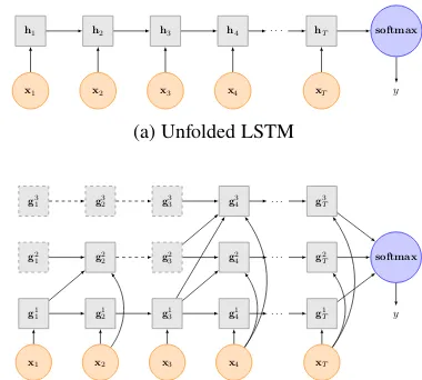
(b) Unfolded MT-LSTM with Fast-to-Slow Feedback Strategy

Figure 2: Illustration of the unfolded LSTM and unfolded MT-LSTM. The dotted node indicates the unit which is inactivated at current time, while the solid node indicates the unit which is activated. The dotted lines indicate the units which kept un-changed, while the solid lines indicate the units which will be updated at the next time step.

LSTM can capture the long-term and short-term dependencies in a sequence. But the long-term dependencies need to be transmitted one-by-one along the sequence. Some important informa-tion could be lost in transmission process for long texts, such as documents. Besides, the error sig-nal is back-propagated through multiple time steps when we use the back-propagation through time (BPTT) (Werbos, 1990) algorithm. The training efficiency could also be low for the long texts. For example, if a valuable feature occurs at the begin of a long document, we need to back-propagate the error through the whole document.

de-layed connections and units operating at different timescales to improve the simple RNN, we sepa-rate the LSTM units into several groups. Different groups capture different timescales dependencies. More formally, the LSTM units are parti-tioned into g groups{G1,· · · , Gg}. Each group

Gk,(1≤k≤g)is activated at different time

pe-riodsTk. Accordingly, the gates and weight

ma-trices are also partitioned to maintain the corre-sponding LSTM groups. The MT-LSTM with just one group is the same to the standard LSTM.

At each time stept, only the groupsGkthat

sat-isfy(tMODTk) = 0 are executed. The choice

of the set of periods Tk ∈ {T1,· · · , Tg} is

arbi-trary. Here, we use the exponential series of peri-ods: groupGk has the period ofTk = 2k−1. The

group G1 is the fastest one and can be executed at every time step, which works like the standard LSTM. The groupGkis the slowest one.

At time stept, the memory cell vector and hid-den state vector of groupGk are calculate in two

cases:

(1) When group Gk is activated at time stept,

the LSMT units of this group are calculated by the following equations:

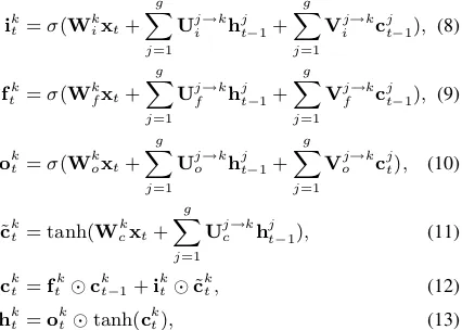
ik

t =σ(Wkixt+ g

∑

j=1 Uj→k

i hjt−1+

g

∑

j=1 Vj→k

i cjt−1), (8)

fk

t =σ(Wkfxt+ g

∑

j=1 Uj→k

f hjt−1+

g

∑

j=1 Vj→k

f cjt−1), (9)

ok

t =σ(Wkoxt+ g

∑

j=1 Uj→k

o hjt−1+

g

∑

j=1 Vj→k

o cjt), (10)

˜ ck

t = tanh(Wkcxt+

g

∑

j=1 Uj→k

c hjt−1), (11) ck

t =ftk⊙ckt−1+ikt ⊙˜ckt, (12)

hkt =okt⊙tanh(ckt), (13)

whereik

t,ftkandokt are the vectors of input gates,

forget gates, and output gates of groupGkat time

steptrespectively;ck

t andhkt are the memory cell

vector and hidden state vector of groupGkat time

steptrespectively.

(2) When groupGkis non-activated at time step

t, its LSMT units keep unchanged.

ck_t =ck_t−1, (14)

hk_t =hk_t−1. (15)

Figure 3 shows the different between the stan-dard LSTM and MT-LSTM.

(a) Fast-to-Slow Strategy (b) Slow-to-Fast Strategy Figure 3: Two feedback strategies of our model. The dashed line shows the feedback connection, and the solid link shows the connection at current time.

4.1 Two Feedback Strategies

The feedback mechanism of LSTM is imple-mented by the recurrent connections from time step t−1 tot. Since the MT-LSTM groups are updated with the different frequencies, we can re-gard the different group as the human memory. The fast-speed groups are short-term memories, while the slow-speed groups are long-term mem-ories. Therefore, an important consideration is what feedback mechanism is between the short-term and long-short-term memories.

For the proposed MT-LSTM, we consider two feedback strategies to define the connectivity pat-terns among the different groups.

Fast-to-Slow (F2S) Strategy Intuitively, when we accumulate the short-term memory to a certain degree, we store some valuable information from the short-term memory into the long-term mem-ory. Therefore, we firstly define a fast to slow strategy, which updates the slower group using the faster group. The connections from group j to groupkexist if and only ifTj ≤Tk. The weight

matrices Uj_i→k, Uj_f→k, Uoj→k, Ujc→k, Vj_i→k, V_fj→k,Voj→kare set to zero whenTj > Tk.

The F2S updating strategy is shown in Figure 3a.

Slow-to-Fast (S2F) Strategy Following the work of (Koutnik et al., 2014), we also investigate another update scheme from slow-speed group to fast-speed group. The motivation is that a long term memory can be “distilled” into a short-term memory. The connections from groupjto groupi

exist only ifTj ≥Ti. The weight matricesUj_i→k, U_fj→k,Uoj→k,Ujc→k,Vji→k,Vfj→k,Vjo→kare set

to zero whenTj < Tk.

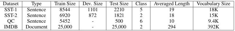
Dataset Type Train Size Dev. Size Test Size Class Averaged Length Vocabulary Size

SST-1 Sentence 8544 1101 2210 5 19 18K

SST-2 Sentence 6920 872 1821 2 18 15K

QC Sentence 5452 - 500 6 10 9.4K

IMDB Document 25,000 - 25,000 2 294 392K

Table 1: Statistics of the four datasets used in this paper.

4.2 Dynamic Selection of the Number of the MT-LSTM Unit Groups

Another consideration is how many groups need to be used. An intuitive way is that we need more groups for long texts than short texts. The number of the group depends the length of the texts.

Here, we use a simple dynamic strategy to choose the maximum number of groups, and then the bestgis chosen as a hyperparameter according to different tasks. The upper bound of the number of groups is calculated by

g= log₂L−1, (16) whereLis the average length of the corpus. Thus, the slowest group is activated at least twice. 5 Training

In each of the experiments, the hidden layer at the last moment has a fully connected layer fol-lowed by a softmax non-linear layer that predicts the probability distribution over classes given the input sentence. The network is trained to min-imise the cross-entropy of the predicted and true distributions; the objective includes an L2 regu-larization term over the parameters. The network is trained with backpropagation and the gradient-based optimization is performed using the Ada-grad update rule (Duchi et al., 2011).

The back propagation of the error propagation is similar to LSTM as well. The only difference is that the error propagates only from groups that were executed at time step t. The error of non-activated groups gets copied back in time (simi-larly to copying the activations of nodes not ac-tivated at the time step t during the correspond-ing forward pass), where it is added to the back-propagated error.

6 Experiments

In this section, we investigate the empirical per-formances of our proposed MT-LSTM model on four benchmark datasets for sentence and docu-ment classification and then compare it to other competitor models.

6.1 Datasets

We evaluate our model on four different datasets. The first three datasets are sentence-level, and the last dataset is document-level. The detailed statis-tics about the four datasets are listed in Table 1. Each dataset is briefly described as follows.

• SST-1 The movie reviews with five classes (negative, somewhat negative, neutral, some-what positive, positive) in the Stanford Senti-ment Treebank1_{(Socher et al., 2013).}

• SST-2 The movie reviews with binary classes. It is also from the Stanford Senti-ment Treebank.

• QC The TREC questions dataset2 _involves

six different question types, e.g. whether the question is about a location, about a person or about some numeric information (Li and Roth, 2002).

• IMDB The IMDB dataset3 _{consists of}

100,000 movie reviews with binary classes (Maas et al., 2011). One key aspect of this dataset is that each movie review has several sentences.

6.2 Competitor Models

We compare our model with the following models:

• NB-SVMandMNB. Naive Bayes SVM and Multinomial Naive Bayes with uni and bi-gram features (Wang and Manning, 2012). • NBOWThe NBOW sums the word vectors

and applies a non-linearity followed by a softmax classification layer.

• RAE Recursive Autoencoders with pre-trained word vectors from Wikipedia (Socher et al., 2011b).

• MV-RNN Matrix-Vector Recursive Neural Network with parse trees (Socher et al., 2012).

1_{http://nlp.stanford.edu/sentiment.}

2_{http://cogcomp.cs.illinois.edu/Data/}

QA/QC/.

3_{http://ai.stanford.edu/˜amaas/data/}

SST-1 SST-2 QC IMDB Embedding size 100 100 100 100 hidden layer size 60 60 55 100 Initial learning rate 0.1 0.1 0.1 0.1 Regularization 10−5 ₁₀−5 ₁₀−5 ₁₀−5

Number of Groups 3 3 3 5

Table 2: Hyper-parameter settings for the LSTM and MT-LSTM.

• RNTN Recursive Neural Tensor Network with tensor-based feature function and parse trees (Socher et al., 2013).

• AdaSentSelf-adaptive hierarchical sentence model with gated mechanism (Zhao et al., 2015).

• DCNNDynamic Convolutional Neural Net-work with dynamic k-max pooling (Kalch-brenner et al., 2014).

• CNN-non-static and CNN-multichannel Convolutional Neural Network (Kim, 2014). • PV Logistic regression on top of paragraph

vectors (Le and Mikolov, 2014). Here, we use the popular open source implementation of PV in Gensim4_.

• LSTMThe standard LSTM for text classifi-cation. We use the implementation of Graves (2013). The unfolded illustration is shown in Figure 2a.

6.3 Hyperparameters and Training

In all of our experiments, the word embeddings are trained using word2vec (Mikolov et al., 2013a) on the Wikipedia corpus (1B words). The vocabu-lary size is about 500,000. The the word embed-dings are fine-tuned during training to improve the performance (Collobert et al., 2011). The other parameters are initialized by randomly sampling from uniform distribution in [-0.1, 0.1]. The hy-perparameters which achieve the best performance on the development set will be chosen for the fi-nal evaluation. For datasets without development set, we use 10-fold cross-validation (CV) instead. The final hyper-parameters for the LSTM and MT-LSTM are set as Figure 2.

6.4 Results

Table 3 shows the classification accuracies of the standard LSTM, MT-LSTM compared with the competitor models.

Firstly, we compare two feedback strategies of MT-LSTM. The fast-to-slow feedback

strat-4_{https://github.com/piskvorky/gensim/}

1 2 3 4 5 6 7 8 0.5

0.6 0.7 0.8 0.9

Number of Iteration

A

cc.(%)

LSTM MT-LSTM

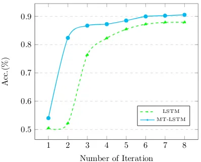
Figure 4: Convergence Speeds on IMDB dataset.

egy (MT-LSTM (F2S)) is better than the slow-to-fast strategy (MT-LSTM (S2F)), which indicates that MT-LSTM benefits from periodically stor-ing some valuable information “purified” from the short-term memory into the long-term memory. In the following discussion, we use fast-to-slow feed-back strategy as the default setting of MT-LSTM.

Compared with the standard LSTM, MT-LSTM results in significantly improvements with the same size of hidden layers.

MT-LSTM outperforms the competitor models on the SST-1, QC and IMDB datasets, and is close to the two best CNN based models on the SST-2 dataset. But MT-LSTM uses much fewer param-eters than the CNN based models. The number of parameters of LSTM range from 10K to 40K while the number of parameters is about 400K in CNN.

Moreover, MT-LSTM can not only handle short texts, but can model long texts in classification task.

trans-Model SST-1 SST-2 QC IMDB NBOW (Kalchbrenner et al., 2014) 42.4 80.5 88.2 -RAE (Socher et al., 2011b) 43.2 82.4 - -MV-RNN (Socher et al., 2012) 44.4 82.9 - -RNTN (Socher et al., 2013) 45.7 85.4 - -DCNN (Kalchbrenner et al., 2014) 48.5 86.8 93.0 -CNN-non-static (Kim, 2014) 48.0 87.2 93.6 -CNN-multichannel (Kim, 2014) 47.4 88.1 92.2

-AdaSent (Zhao et al., 2015) - - 92.4

-NBSVM (Wang and Manning, 2012) - - - 91.2

MNB (Wang and Manning, 2012) - - - 86.6

Two-level DCNN (Denil et al., 2014) - - - 89.4 PV (Le and Mikolov, 2014) 44.6* 82.7* 91.8* 91.7*

LSTM 47.9 85.8 91.3 88.5

MT-LSTM (S2F) 48.9 86.7 93.3 90.2

MT-LSTM (F2S) 49.1 87.2 94.4 92.1

Table 3: Results of our MT-LSTM model against state-of-the-art neural models. All the results without marks are reported in the corresponding paper.

1 2 3 4 5

44.5 45 45.5 46 46.5 47

(a) SST-1

1 2 3 4 5

84.6 84.8 85 85.2 85.4 85.6 85.8

(b) SST-2

1 2 3 4

90 90.5 91 91.5 92 92.5

(c) QC

1 2 3 4 5 6 8 88.5

89 89.5 90

(d) IMDB

Figure 5: Performances of our model with the dif-ferent numbers of memory groupsgon four devel-opment datasets: SST-1,SST-2, QC, and IMDB. Y-axis represents the accuracy(%), and X-axis rep-resents different numbers of memory groups. All memory groups share a fixed-size memory layer

h, and here we seth=120.

form embeddings for the words in each sentence into an embedding for the entire sentence. The second level uses another DCNN to transform sen-tence embeddings from the first level into a single embedding vector that represents the entire docu-ment. However, their result is unsatisfactory and they reported that the IMDB dataset is too small to train a CNN model.

The standard LSTM has an advantage to model documents due to its simplification. However, it is also difficult to train LSTM since the error signals need to be back-propagated over a long distance

with the BPTT algorithm.

Our MT-LSTM can alleviate this problem with multiple timescale memories. The experiment on IMDB dataset demonstrates this advantage. MT-LSTM achieves the accuracy of 92.1% , which are better than the other models.

Moreover, MT-LSTM converges at a faster rate than the standard LSTM. Figure 4 plots the con-vergence on the IMDB dataset. In practice, MT-LSTM is approximately three times faster than the standard LSTM since the hidden states of low-speed group often keep unchanged and need not to be re-calculated at each time step.

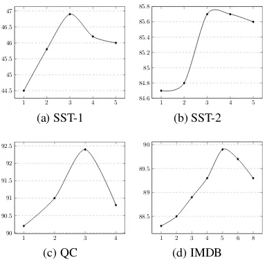
Impact of the Different Number of Memory Groups In our model, the number of memory groups is a hyperparameter. Here we plotted the accuracy curves of our model with the different numbers of memory groups in Figure 5 to show its impacts on the four datasets.

When the length of text (SST-1, SST-2 and QC) is small, not all memory groups can be acti-vated if we set too many groups, which may harm the performance. When dealing with the long texts (IMBD), more groups lead to a better per-formance. The performance can be improved with the increase of the number of memory groups.

<s> Is this progress ? </s> 0.2

0.3 0.4 0.5

LSTM MT-LSTM

<s> He ’d create a movie better than this . </s> 0

0.2 0.4 0.6 0.8

LSTM MT-LSTM

<s> It ’s not exactly a gourmet meal but the fare is fair , even coming from the drive . </s>

0 0.2 0.4 0.6 0.8

LSTM MT-LSTM

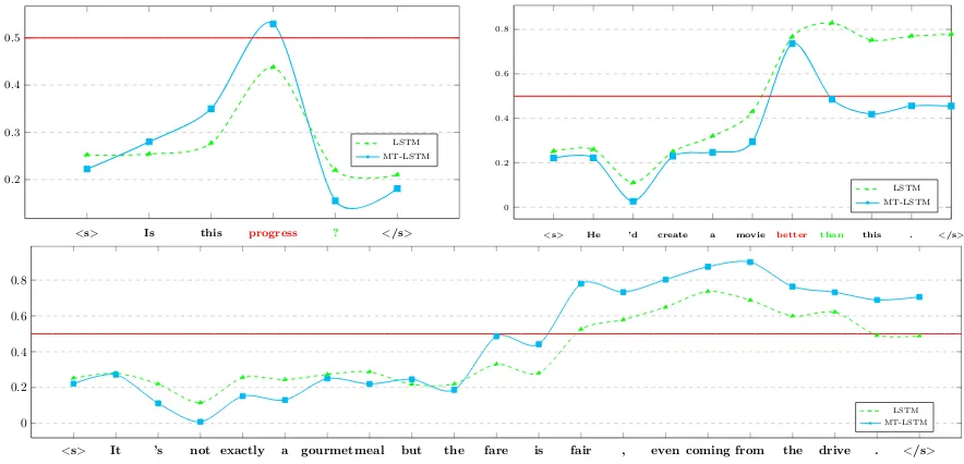
Figure 6: The dynamical changes of the predicted sentiment score over time. Y-axis represents the sentiment score, while X-axis represents the input words in chronological order. The red horizontal line gives a border between the positive and negative sentiments.

6.5 Case Study

To get an intuitive understanding of what is hap-pening when we use LSTM or MT-LSTM to pre-dict the class of text, we design an experiment to analyze the output of LSTM and MT-LSTM at each time step.

We sample three sentences from the SST-2 test dataset, and the dynamical changes of the pre-dicted sentiment score over time are shown in Fig-ure 6. It is intriguing to notice that our model can handle the rhetorical question well.

The first sentence “Is this progress ?” has a negative sentiment. Although the word

“progress” is positive, our model can adjust the

sentiment correctly after seeing the question mark “?”, and finally gets a correct prediction.

The second sentence “He ’d create a

movie better than this .” also has a

negative sentiment. The word “better” is posi-tive. Our model finally gets a correct negative pre-diction after seeing “than this”, while LSTM gets a wrong prediction.

The third sentence “ It ’s not exactly a gourmet meal but fare is fair

, even coming from the drive .”

is positive and has more complicated semantic composition. Our model can still capture the useful long-term features and gets the correct prediction, while LSTM does not work well.

7 Related Work

There are many previous works to model the variable-length text as a fixed-length vector. Spe-cific to text classification task, most of the mod-els cannot deal with the texts of several sen-tences (paragraphs, documents), such as MV-RNN (Socher et al., 2012), RNTN (Socher et al., 2013), CNN (Kim, 2014), AdaSent (Zhao et al., 2015), and so on. The simple neural bag-of-words model can deal with long texts, but it loses the word order information. PV (Le and Mikolov, 2014) works in unsupervised way, and the learned vector cannot be fine-tuned on the specific task.

Our proposed MT-LSTM can handle short texts as well as long texts in classification task.

8 Conclusion

In this paper, we introduce the MT-LSTM, a gen-eralization of LSTMs to capture the information with different timescales. MT-LSTM can well model both short and long texts. With the multi-ple different timescale memories. Intuitively, MT-LSTM easily carries the crucial information over a long distance. Another advantage of MT-LSTM is that the training speed is faster than the standard LSTM (approximately three times faster in prac-tice).

Acknowledgments

We would like to thank the anonymous review-ers for their valuable comments. This work was partially funded by the National Natural Science Foundation of China (61472088, 61473092), Na-tional High Technology Research and Develop-ment Program of China (2015AA015408), Shang-hai Science and Technology Development Funds (14ZR1403200).

References

Yoshua Bengio, Patrice Simard, and Paolo Frasconi. 1994. Learning long-term dependencies with gra-dient descent is difficult. Neural Networks, IEEE Transactions on, 5(2):157–166.

Yoshua Bengio, R´ejean Ducharme, Pascal Vincent, and Christian Janvin. 2003. A neural probabilistic lan-guage model. The Journal of Machine Learning Re-search, 3:1137–1155.

Xinchi Chen, Xipeng Qiu, Chenxi Zhu, Pengfei Liu, and Xuanjing Huang. 2015. Long short-term mem-ory neural networks for chinese word segmenta-tion. InProceedings of the Conference on Empirical Methods in Natural Language Processing.

Kyunghyun Cho, Bart van Merrienboer, Caglar Gul-cehre, Fethi Bougares, Holger Schwenk, and Yoshua Bengio. 2014. Learning phrase representations using rnn encoder-decoder for statistical machine translation. InProceedings of EMNLP.

Junyoung Chung, Caglar Gulcehre, KyungHyun Cho, and Yoshua Bengio. 2014. Empirical evaluation of gated recurrent neural networks on sequence model-ing. arXiv preprint arXiv:1412.3555.

Ronan Collobert, Jason Weston, L´eon Bottou, Michael Karlen, Koray Kavukcuoglu, and Pavel Kuksa. 2011. Natural language processing (almost) from scratch. The Journal of Machine Learning Re-search, 12:2493–2537.

Misha Denil, Alban Demiraj, Nal Kalchbrenner, Phil Blunsom, and Nando de Freitas. 2014. Modelling, visualising and summarising documents with a sin-gle convolutional neural network. arXiv preprint arXiv:1406.3830.

John Duchi, Elad Hazan, and Yoram Singer. 2011. Adaptive subgradient methods for online learning and stochastic optimization. The Journal of Ma-chine Learning Research, 12:2121–2159.

Salah El Hihi and Yoshua Bengio. 1995. Hierarchical recurrent neural networks for long-term dependen-cies. InNIPS, pages 493–499. Citeseer.

Jeffrey L Elman. 1990. Finding structure in time. Cognitive science, 14(2):179–211.

Alex Graves. 2013. Generating sequences with recurrent neural networks. arXiv preprint arXiv:1308.0850.

Sepp Hochreiter and J¨urgen Schmidhuber. 1997. Long short-term memory. Neural computation, 9(8):1735–1780.

Sepp Hochreiter, Yoshua Bengio, Paolo Frasconi, and J¨urgen Schmidhuber. 2001. Gradient flow in recur-rent nets: the difficulty of learning long-term depen-dencies.

Baotian Hu, Zhengdong Lu, Hang Li, and Qingcai Chen. 2014. Convolutional neural network archi-tectures for matching natural language sentences. InAdvances in Neural Information Processing Sys-tems.

Nal Kalchbrenner, Edward Grefenstette, and Phil Blun-som. 2014. A convolutional neural network for modelling sentences. InProceedings of ACL. Yoon Kim. 2014. Convolutional neural

net-works for sentence classification. arXiv preprint arXiv:1408.5882.

Jan Koutnik, Klaus Greff, Faustino Gomez, and Juer-gen Schmidhuber. 2014. A clockwork rnn. In Pro-ceedings of The 31st International Conference on Machine Learning, pages 1863–1871.

Quoc V. Le and Tomas Mikolov. 2014. Distributed representations of sentences and documents. In Pro-ceedings of ICML.

Xin Li and Dan Roth. 2002. Learning question classi-fiers. InProceedings of the 19th International Con-ference on Computational Linguistics, pages 556– 562.

Andrew L Maas, Raymond E Daly, Peter T Pham, Dan Huang, Andrew Y Ng, and Christopher Potts. 2011. Learning word vectors for sentiment analysis. In Proceedings of the 49th Annual Meeting of the Asso-ciation for Computational Linguistics: Human Lan-guage Technologies-Volume 1, pages 142–150. As-sociation for Computational Linguistics.

Tomas Mikolov, Martin Karafi´at, Lukas Burget, Jan Cernock`y, and Sanjeev Khudanpur. 2010. Recur-rent neural network based language model. In IN-TERSPEECH.

Tomas Mikolov, Kai Chen, Greg Corrado, and Jef-frey Dean. 2013a. Efficient estimation of word representations in vector space. arXiv preprint arXiv:1301.3781.

Tomas Mikolov, Ilya Sutskever, Kai Chen, Greg S Cor-rado, and Jeff Dean. 2013b. Distributed representa-tions of words and phrases and their compositional-ity. InNIPS, pages 3111–3119.

Jordan B Pollack. 1990. Recursive distributed repre-sentations.Artificial Intelligence, 46(1):77–105. Richard Socher, Cliff C Lin, Chris Manning, and

An-drew Y Ng. 2011a. Parsing natural scenes and nat-ural language with recursive nenat-ural networks. In Proceedings of the 28th International Conference on Machine Learning (ICML-11), pages 129–136. Richard Socher, Jeffrey Pennington, Eric H Huang,

Andrew Y Ng, and Christopher D Manning. 2011b. Semi-supervised recursive autoencoders for predict-ing sentiment distributions. In Proceedings of the Conference on Empirical Methods in Natural Lan-guage Processing, pages 151–161.

Richard Socher, Brody Huval, Christopher D Manning, and Andrew Y Ng. 2012. Semantic compositional-ity through recursive matrix-vector spaces. In Pro-ceedings of the 2012 Joint Conference on Empiri-cal Methods in Natural Language Processing and Computational Natural Language Learning, pages 1201–1211.

Richard Socher, Alex Perelygin, Jean Y Wu, Jason Chuang, Christopher D Manning, Andrew Y Ng, and Christopher Potts. 2013. Recursive deep mod-els for semantic compositionality over a sentiment treebank. In Proceedings of the conference on empirical methods in natural language processing (EMNLP).

Ilya Sutskever, Oriol Vinyals, and Quoc VV Le. 2014. Sequence to sequence learning with neural net-works. InAdvances in Neural Information Process-ing Systems, pages 3104–3112.

Joseph Turian, Lev Ratinov, and Yoshua Bengio. 2010. Word representations: a simple and general method for semi-supervised learning. InProceedings of the 48th annual meeting of the association for compu-tational linguistics, pages 384–394. Association for Computational Linguistics.

Sida Wang and Christopher D Manning. 2012. Base-lines and bigrams: Simple, good sentiment and topic classification. In Proceedings of the 50th Annual Meeting of the Association for Computational Lin-guistics: Short Papers-Volume 2, pages 90–94. As-sociation for Computational Linguistics.

Paul J Werbos. 1990. Backpropagation through time: what it does and how to do it. Proceedings of the IEEE, 78(10):1550–1560.

Kaisheng Yao, Baolin Peng, Yu Zhang, Dong Yu, Ge-offrey Zweig, and Yangyang Shi. 2014. Spoken lan-guage understanding using long short-term memory neural networks. IEEE SLT.