A Comparison of Criteria for Maximum Entropy/ Minimum Divergence Feature Selection

A Comparison of Criteria

for Maximum Entropy / Minimum Divergence

Feature Selection

Adam Berger

Carnegie Mellon University School of Computer Science

Pittsburgh, PA 15232 aberger0cs.cmu.edu

Abstract

In this paper we study the gain, a naturally-arising statistic from the theory of MEMD modeling [2], as a figure of merit for selecting features for an MEMD language model. We compare the gain with two popular alternatives-empirical activation and mutual information-and argue that the gain is the preferred statistic, on the grounds that it directly measures a fea-ture's contribution to improving upon the base modeL

Introduction

Maximum entropy / minimum divergence (MEMD) modeling is a powerful technique for building statisti-cal models of linguistic phenomena. It has been applied to problems as diverse as machine translation [2], pars-ing [10], word morphology [5] and language modelpars-ing [6, 11, 3, 9]. The heart of the method is to ~ljoose a collection of informative features, each encodi'llg some linguistically significant event, and then to incorporate these features into a family of conditional models.

A fundamental issue in applying this technique is the criterion used to select features. The work described in (3], for instance, incorporates every feature which either appears with above-threshold count in a training cor-pus, or which exhibits high mutual information. In [11] and [1], the authors select features based on a mutual information statistic. As we argue below, both these methods have drawbacks.

In this paper, we examine a statistic for selecting MEMD model features, called the gain. The gain was introduced in [4], and studied in greater detail in [5] and [2]. We present intuition, theory and experimen-tal results for this statistic, as a criterion for selecting features for an MEMD language model. We believe our work marks the first time it has been used in MEMD language modeling, and the first side-by-side compar-ison with other selection criteria. Though our experi-mental results concern language models exclusively, we note that the gain can be used to select features for any MEMD model on a discrete space.

The language model we present is based on depen-dency grammars. It is similar to, but extends upon, the work reported in [3]. Two important differences between that work and ours are that ours is a true

Harry Printz

IBM

Watson Research Center Yorktown Heights, NY 10598

[email protected]

minimum-divergence model, and ours incorporates both link and trigger features.

The paper is organized as follows. In Section Struc-ture of the Model we give a briefreview of MEMD models in general, and of our dependency grammar model in particular. In Section Linguistic Features we describe and motivate the types of features we chose to inves-tigate. In Section Expe1'imental Setup we describe our experimental procedure. In Section Selection of Fea-tU?·es we discuss feature selection; it is here that we develop the notion of gain. In Section Additivity of the Gain we discuss the additivity of gain, which measures the extent to which features contribute independently

tO

a modeL In Section Tests and Results we report our test results. Section Summary concludes the paper.

Structure of the Model

Use of a Linkage

Let

's

=

w0 .•. wN be the sentence in question, and let

K(S)

or just

K

stand for its linkage. A linkage is a planar graph, in which the nodes are the words of S, and the edges connect linguistically related word pairs. A typical sentenceS, with its linkage J(, appears in Figure 1. The relationship between the linkage of a sentence, and the familiar notion of a parse tree, is described in Section Experimental Setup below.

<s>

0

one (}oz·e~ b(uimia cr~a'!"' pies <Is>

2 3 4 5 6 7 8 9

Figure 1: A Sentence S and its Linkage K. The shaded area represents the history h7

, which is the

conditioning information available to the model at position 7. h 7 consists of the complete linkage K, and words w0 through w6 _inclusive.

Our model, written

P(S

I

K),

is not a language model proper, since it is conditioned upon the linkage. In principle we can recover

P(S)

as

I;K

P(S

I

K)P(K);

since K itself depends upon S, the model cannot be ap-plied incrementally, for instance in a real-time speech recognition system. However, such a model can be used to select from a list of complete sentences.

The value P(S

I

K) computed by our model is formed in the usual way as the product of individual word prob-abilities; that is

N N

P(S

I

K)

=

ITp(w'

I

w~-1K)

=

ITp(w'

I

h'). (1)

i=O i=O

Here we have written hi :::: (w~~ 1, K) for the history at position i; this is the information the model may use when predicting the next word. Here and below the notation

wi,

with i

S

j, stands for the word sequence wi , , . wj. Thus for the models in this paper, the

his-tory consists of the words w0 _{. .. wi-I, plus the complete} linkage K.

Fundamentals of MEMD Models

The individual word probabilities p(w'

I

h') appearing in equation (1) above are determined by a minimum divergence model. Here we review of the fundamentals of such models; a thorough description appears in ref-erence

[2].

As above, let w stand for the word or fu·ture to be pre-dicted, and let h stand for the history upon which this prediction is based. Suppose that

f(

w h) is a binary-valued indicator function of some linguistic event. For instance,

f

may take the value 1 when the most recent word of h is the definite article the and the word w is any noun; otherwise

f

is 0. Or

f

might be 1 when h contains the word dog in any location and w is the word barked. Any such function f( w h) is called a binary

fea-ture function; clearly we can invent a large number of such functions.

Now suppose C is a large corpus. C can be regarded as a very long sequence of word-history pairs wi hi, where w~ is the word at position i and ht is the history at that position. We can use C to define the empirical expectation

E,;[J]

of any feature function

J;

it is given by

E,;[f]

=I:

J(w' hi)/N (2)

where i runs over all the positions of the corpus, and N is the number of positions. The sum AJ

=I;, f(wi

h')

is called the empirical activation of the feature f; it is the number of corpus positions where the feature is active (attains the value 1).

Finally, let q(w

I

h) be some selected statistical lan-guage model, for instance a trigram model. We call q the base model. When q is a trigram, it predicts w based exclusively upon the two most recent words appearing in h. Note however that an arbitrary feature function

f

can inspect any word of h, or the linkage itself if it com-prises part of h. It is the enlarged scope of information available to

f

that we hope to exploit.

We can now enunciate the principle of minimum di-vergence modeling. Let

f

=

(J, ... fM) be a vector of binary feature functions, with a known vector of em-pirical expectations

(Eft[h] ...

Ep[fM ]). We seek the model p(w

I

h) of minimal Kullback-Liebler divergence from the base model q(w

I

h), subject to the constraint that

That is, the expectation of each

fi,

according to the model p, must equal its empirically observed expecta-tion on the corpus C.

By familiar manipulations with Lagrange multipliers, as detailed in [2], the solution to this problem can be shown to be

p(w

I

h)= - -

1

-q(w

I

h)e•·f(w h)

(4)

Z(ii h)

where

Z(ii h)=

I;

q(w

I

h)e".f(w h)_

₍₅₎

wEV

Here

f(

w h) is a vector of Os and 1s, depending upon the value of each feature function at the point w h. Likewise & is a vector of real-valued exponents, which are adjusted during the training of the model so that equation (3) holds. V is a fixed vocabulary of words, and Z( & h) is a normalizing value, computed according to equation

(5).

Finally q(w

I

h) is the base model, which represents our nominal prediction of w from h. When q is the constant function 1/jVI, the resulting model p is called a maximum entropy model; when q is non-constant, p is called a minimum diveTgence model. However the defining equations (4, 5) are the same, regardless of the nomenclature.

Use of a Base Model

In the work reported here, the base model q is decid-edly not a constant: it is a linearly-interpolated trigram model, trained on a corpus of 44,761,334 words. This approach, while not novel [1], is one of the key depar-tures of our work from [3].

This departure is significant for three reasons. First, it gives us a computationally efficient way to incorpo-rate a large amount of valuable information into our model. 'l'o put this another way, we already know that the 14,617,943 trigrams, 3,931,078 bigrams and 56,687 unigrams that together determine q are useful linguistic predictors. But if we should try to incorporate each of these word-grams into a pure maximum entropy frame-work, via its corresponding feature function, we would be faced with an intractable computational problem.

Third, using a trigram base model raises a new and challenging version of the feature selection problem. How can we determine which features, when incorpo-rated into the model, will actually yield an advance upon the trigram model? This is the central problem of this paper, which we proceed to address by using the gain statistic.

Linguistic Features

We now take up the question of how to exploit the information in the history hi to more accurately esti-mate the probability of word

w'.

We remind the reader that the base model already provides such an estimate, q(w'

I

h'). But because in this case q is a trigram model, it discards all of hi except the two most recent words, wi-2_{wi-l. Our aim is to find informative binary}

feature functions f(w'

h')

that are clues to especially likely or unlikely values of

w'.

We chose to use two different kinds of features: triggers and links.

Trigger Features

As every speaker of English is aware, the appearance of one given word in a sentence is often strong evidence that another particular word will follow. For instance, knowing that computer appeared among the words of hi, one might expect that nerds is more likely than nor-mal to appear among the remaining words of the sen-tence. Some words are in fact good predictors of them-selves: seeing Japanese once in a sentence raises the likelihood it will appear again later. Word pairs such as these, where the appearance of the first is s.tfongly correlated with the subsequent appearance of ·'the sec-ond, are called trigger pairs [1, 11]. Note that ,the trig-ger property is not necessarily symmetric: we would expect a left parenthesis { to trigger a right parenthesis }, but not the other way around.

Our model incorporates these relationships through trigger features. Let u, v be some trigger pair. A trigger feature fuv is defined as

fuv(w h)= {

6

_otherwise if w

=

v and h3 u with

luvl2:

dmin

(6)

Here h 3 u, read "h contains u/1 _{means that u appears}

somewhere in the word sequence of h. The notation

luvl 2:

dmin means that the span of this pair, defined as the number of words from u to v, including u and v themselves, is not less than a predetermined threshold dmin· Throughout this work we have used dmin ::::: 3.

Link Features

One shortcoming of trigger features is their profligacy. In a model built with the feature !computer nerds1 an

ap-pearance of computer will boost the probability of nerds at every position at distance dmin or more to its right. This will be so whether or not a position is a linguis-tically appropriate site for nerds. Moreover, if a model contains a large number of trigger features, there will

be many triggered words at each position, and their heightened probabilities will tend to wash each other out.

For instance consider the sentence of Figure 2. The plausible trigger feature !stocks rose will boost the prob-ability of rose at every word from position 4 onward, in particular at position 6. But here the acoustically confusable word woes appears, and so increasing the probability of rose at this position could yield an error. Thus the boost that !stocks ?'ose gives to rose, which we desire in position

8,

is just as clearly not desired in position 6. Unfortunately the trigger is blind to the distinction between these two sites, and it boosts rose in both places.

<s> Nasdaq stocks , despite Asian woes rose shmply . <Is>

0 I 2 3 4 5 6 7 8 9 10 II

Figure 2: Links versus Triggers. The trigger fea-ture for stocks and rose boosts the probability of

rose at each position from 4 to 11, inclusive. The link feature also boosts rose, but only at positions 4 and 8. The linkage shown here is the actual one

computed by our parser.

These considerations have led us and others to con-sider features that use the linkage. The aim is to focus the effect of words in the history upon the particular positions that are appropriate for them to influence. Figu:re 2 shows how the linkage of this sentence con-nects stocks1 the headword of the subject noun phrase,

with i'ose, the main verb of the sentence; note there is no such link from stocks to woes. These are precisely the linguistic facts that we wish to exploit, using an ap-propriate feature function. To do so, we will construct a feature function that (like a trigger) turns on only for a given word pair, and in addition only when the named words are connected by an arc of the linkage.

Because such features depend upon the the linkage of the sentence, we refer to them as link features. Such a feature f,.... _uv 1 for words u and v, is defined as

J~(wh)=

{ 1

u v 0

if w

=

v and h3uv with

luvl 2:

dmin otherwise

(7)

The notation h :Ju,...,v, read "h contains u, linking v/1

means that word u appears in the history's word se-quence, that an arc of K connects u with the current position, and that word v appears in the current po-sition. In the example given above, the link feature

f

~ attains the value 1 at position 8 only.

stocks rose

Experimental Setup

Here we describe the

work in this paper.

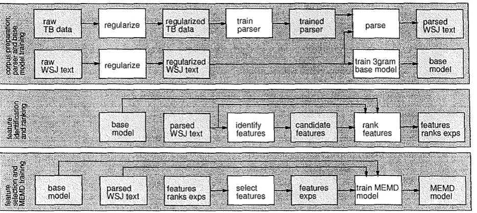
computation that underlies Figure 3 is a schematic of

complete computation, which divides into three phases: (1) prepare the corpus and train a parser and base model, (2) identify and rank features, and (3) select features and train an MEMD model. Our experiments, which we report later, concerned phases (2) and (3) only. We include a discussion of phase ( 1) for com-pleteness, and to place our experiments in context.

In the first phase we trained a parser and base model, and parsed the corpus text. By parsed we mean that for each sentence S of the corpus text T, we have its linkage

f( ( S) at our disposal. The parser we trained and then used was a modified version of the decision- tree parser described in [7]. Our parser training corpus consisted of 990,145 words of Tree bank Release II data, and our base model corpus consisted of 44,761,334 words of Wall Street Journal data, both prepared by the Linguistic Data Consortium.

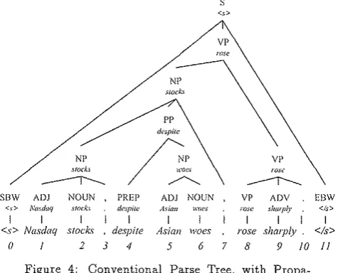
This parser constructs a conventional parse tree. Since we needed linkages, we used the method of head-word propagation to create them from the parser out-put; we now explain this method. To each parse tree we apply a small collection of headword propagation rules, which operate leaves-to-root. The result is a tree la-beled with a headword at each node, where each head-word is selected from the headhead-words of a node's chil-clren. (At the leaves, each word is its own headword.) The desired linkage is then obtained by drawing an arc from the headword of each child node to the headword ofits parent, excluding self-loops. A conventional parse tree for the sentence of Figure 2 above, labeled with propagated headwords, appears in Figure 4.

SBW

<.,>

<s> (I

s

ADJ NOUN PREP ADJ NOUN yp ADV

Nmdaq .\'lock.\ de>piw A,,·,·au \WJ('.\' !'OS<~ sluuply

I I I I

Nasdaq stocks despite Asian woes rose shmply

2 3 4 5 6 7 8 9 10

Figure 4: Conventional Parse Tree, with Propa-gated Headwords. The text explains how this head-word-labelled tree can be transformed into the link-age of Figure 2.

EBW

<Is>

<Is>

11

For the base model q1 we chose to use a linearly

inter-polated trigram language model, built from the same regularized WSJ corpus as the dependency grammar model itself.

In the second processing phase we identified and ranked features. The details of this phase, and in par-ticular the figure of merit used for ranking1 are the

sub-ject of Section Selection of Features. Here we explain its place in the overall scheme. By inspecting the parsed corpus C, we identify a set F of trigger and link candi-date features. These are then ranked according to the chosen statistic. In this paper we advocate the use of the gain as the rank statistic. The gain depends upon both the corpus and the base model, and for this rea-son these are shown as inputs to the box rank features in Figure 3. The output is the same set of candidate features, ranked according to the figure of merit. It

happens that the gain computation also yields initial estimates of the MEMD exponents; abbreviated exps in the figure.

In the final phase of processing, we inspected the ranked list of features and selected those to incorpo-rate into the model. We then used the selected fea-tures, their initial exponent estimates, the corpus1 and

the base model to train the MEMD model. Different choices of features yield different models; Section Tests and Results below gives details and performance of the various models we built.

Selection of Features

Once the model's prior and feature types have been chosen-choices generally dictated by computational practicality, and the information available in the traing corpus-the key open issue is which features to in-corporate in the model. In general we cannot and will not want to use every possible feature. For one thing, we usually have too many features to train a model that includes all of them: the processing and memory requirements are just too great. Moreover 1 rescoring

with a model that has a very large number of features is itself time-consuming. Finally1 many features may be

of little predictive value, for they may seldom activate, or may just repeat information that is already present in the prior.

In this section we describe a method for selecting precisely those features of greatest predictive power, over and above the base model q. The key idea of our method is to seek features that improve upon q's pre-dictions of the training corpus itself. The measure of improvement is a statistic called the gain, which we define and motivate below. As we will demonstrate, computing the gain not only yields a principled way of selecting features; it can also be of great help in con-structing the MEMD model that contains the selected features.

Our method proceeds in three steps: candidate iden-tification, ranking, and selection. We now describe each step in greater detail.

Candidate Identification

[image:4.594.56.294.435.627.2]

po-Figure 3: Corpus Preparation, Feature Ranking, and Model Training

tential features for the model. The result of this pass is a candidate feature set1 denoted F. The candidate

features are those that we will rank by gain in the next step.

Nate that one or more criteria may be applied to decide which features, out of the many exhibited in the corpus, are placed into F in the first place. In the work reported here, we scanned the parsed colfus to collect potential features, both triggers and links. Since we were building a model using a trigram prior, we had good reason to believe that adjacent wOrds were well-modeled by this prior, and so we ignored links or triggers of span 2. To keep from being swamped with features of no semantic importance, and which arise purely because the words involved are common ones, we likewise ignored triggers where either word was among the 20 most frequent in the corpus. Moreover we did not include any trigger pair with an empirical activation below 6, nor any link pair with a count below 4.

In this way we collected a total of 538,998 candi-date link features (which were all those passing the cri-teria above) and 1,000,000 candidate trigger features (which were those passing the criteria above, and then the top 1,000,000 when sorted by mutual information). We supplied the resulting candidate set F, containing 1,538,998 features, to the next stage of the feature se-lection process.

Ranking

In this section we will motivate and develop the central feature of this paper, which is the notion of gain. First introduced in [2], and further developed in [5], the gain is a statistic computed for a given feature j, with re-spect to a base model, over some fixed corpus. We will argue that the gain is the appropriate figure of merit

for ranking features.

Motivation At the heart of the issue lie the following two questions. First, how much does a feature

f

aid us in modeling the corpus? Second, to what extent does this feature help us to improve upon the base model? By giving quantitative answers to these questions, we will be led to the gain.

We begin by establishing some notation. Let

P(

C) stand for the probability of the corpus, according to the base model q; that is P(C) =

rr;;:,o

q(w'

I

h'). For the model developed here, this should more properly be written P(T

I

K), where T represents the collected text of the corpus, and K consists of the linkage of each sentence of T. However since our meaning is clear, for typographic simplicity we will use the shorter notation. Now we remind the reader of the connection be-tween MEMD training and maximum-likelihood estima-tion. Suppose we construct an exponential model, from base model q, that contains one single feature f(w

h).

The form of this model will be

Pa(w

I

h)=

Z(~

h) q(w

I

h) eaf(w h) (8)

where Z(a h) is the usual normalizer, and a is a free parameter. For any given value of a, the probabil-ity PJa( C) of the entire corpus C, as predicted by this model, is

N-1

PJa(C)

=

II

Pa•(w'

I

h'). ( 9)

i=:O

The MEMD trained value of a, denoted a*, is determined as

a*= argmaxPJa(C).

(10)

a

[image:5.594.48.516.83.292.2]

This fact is demonstrated in [5], along with a proof that the maximizing a* is unique.

Thus the probability of the complete corpus, accord-ing to the MEMD model p,~, is just Pjo•(C). When the identity of the feature is clear1 we will abbreviate this

by P,~ (C).

We proceed to motivate and define the gain. At many positions of the corpus, the models q and Pa• will yield the same value. But in those positions where they

dis-ag:ree1 we would hope that Pc(•· does a better job1 in

the sense that Po•(wi

I

hi)

>

q(wi

I

hi). That is, we wish that Pa• distributes more probability mass than q on the word that actually appears in corpus position i. The extent to which this occurs is a measure of the predictive value off, the feature that underlies Po•·

Of course, we do not want to gauge the value of

f

by a comparison of models on this or that particular corpus position. But we can judge the overall value of

f

by comparing P,, (C), the probability of the entire corpus according to a model that incorporates both q and /, with P(C), the probability of the entire corpus according to q alone.

VVe can quantify the degree of improvement by

writ-ing

*

1 Po* (C) 1 , 1

a,(cx )

=

N log

P(C)

=

N logP,.(C)- N logP(C).

(11)

We refer to G f ( <>*) as the gain of feature

f.

By the rightmost equality above, the gain measures the im-provement in cross-entropy afforded by

f,

or more sim-ply, the information content of

f.

When it is clear which feature we mean, we will write just

G(

a*) for its gain. Likewise we will write Gj when we don't need to dis-play the exponent. The seemingly ancillary quantity a* is in fact of value, since it is an initial estimate of the feature's associated exponent, and may be used as a starting point in an MEMD training computation that includes this and other features.

Clearly, computing a feature's gain is intimately re-lated to training an MEMD model containing this single feature. But because the model Pcx* involves only one feature, substantial computational speedup is possible. A fast algorithm for computing the gain appears in [8]. The notion of gain extends naturally to a set of fea-tures M. If PM(C) is the corpus probability according to a trained MEMD model built with feature set M, then we define GM

=

(1/N)log(PM(C)/P(C)).

Comparison with Other Criteria A key advan-tage of the gain as a figure of merit is that it overcomes shortcomings of two competing criteria: the feature's empirical activation, and the mutual information of its history with its future. There are clear rationales for both alternatives, but also clear drawbacks.

Selecting by empirical activation ensures that we are choosing features that could significantly reduce the corpus perplexity, for they are active at many corpus positions, and hence can often alter the base model

probability. But there is no guarantee that they change the MEMD model much from the base model, since the selected features might simply express regularities of language that the base model already captures. Of course there is no harm in this, but it does not yield a better model.

Likewise, the mutual information criterion could choose features that coincide with, rather than depart from, the base modeL Moreover this criterion can suffer from inaccurate estimates of its constituent

probabili-ties, when the feature is rare.

The gain remedies these problems. It finds features that cause the MEMD model to depart, in a favorable way, from the base modeL And if a feature is rarel it is ignored, unless it is very valuable in those cases where it appears.

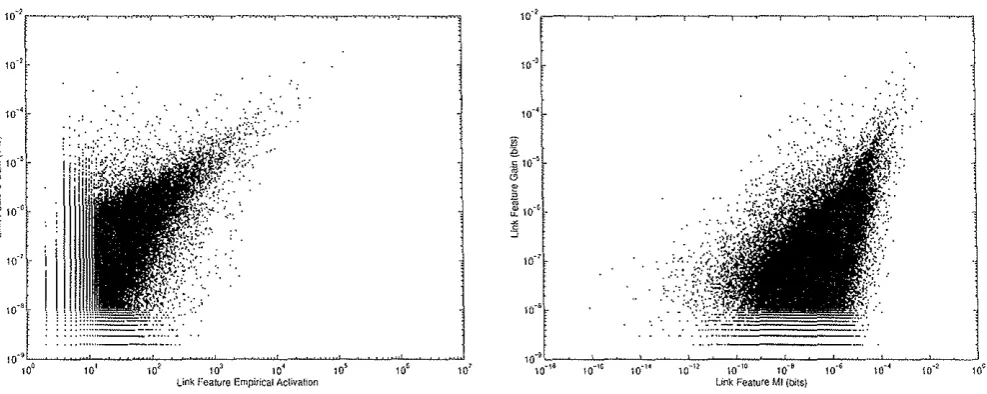
To test this claim, we computed the gain, empiri-cal activation, and mutual information of the 538,998 candidate link features that we collected earlier from our corpus. We then plotted the gain against empir-ical activation, and against mutual information; these plots appear in Figure 5. It is clear that gain is only weakly correlated with these competing statistics. In Section Models Trained below, we compare the perplex-ities of models built by selecting features with these three criteria.

Final Selection

Ranking places the features ofF in order, from most to least gainful. However, though it is clear that we wish to choose features from F in rank order, say retaining the top 10,000 or 100,000 features, the ranking algorithm does not indicate how many features to select. Thus this last step-choosing where in the ranked list to draw the line-must be decided by hand by the modeler.

Since part of our aim was to compare the relative value of link and trigger features, we elected to build models containing the top T triggers and the top L

links, for various values of T and L. We also built a model in which we simply retained the top 10,000 features by rank, without regard to their type.

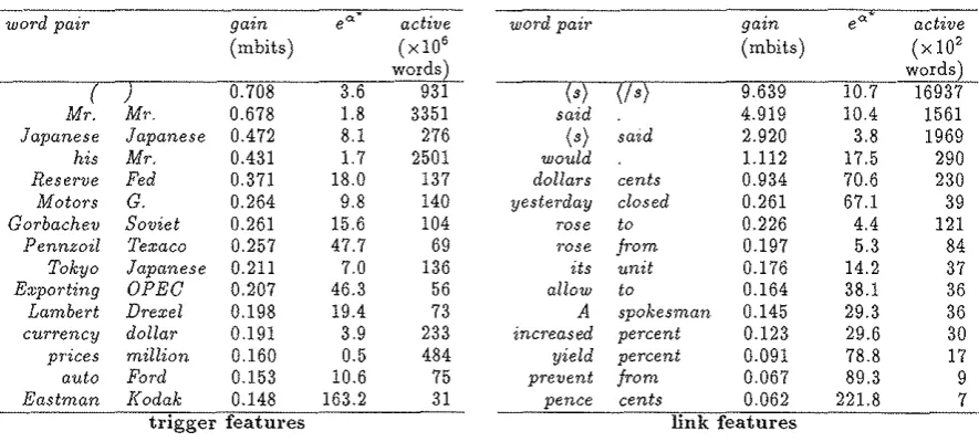
For illustration, we provide in Table 1 a list of 25 selected trigger and link features, of the 1,538,998 in F,

ranked by gain. The table also gives the value of<>* for each feature f; this number is reported as eo:~-, since this roughly corresponds the probability boost the future of each feature receives, when the feature is active.

Comparison with Feature Induction

w' 10... .~ ~ .~ .~ ~ ·~ .~ -~~-.~ .~ .~

l.i~k Feature Ml (bits)

Figure 5: Comparison of 2Link Feature Gain with Empirical Activation and Mutual Information. Left: Scatterplot of feature gain against empirical activation. Right: Scatterplot of feature gain against mutual information.

iterative algorithm for choosing features; it selects one new feature on each iteration. One iteration consists of ( 1) complete training of an MEMD model using a current set of selected features, initially empty, (2) ranking all remaining candidates against this just-trained model, and

(3)

removing the single top-ranking feature from the candidate set, and adding it to the set of selected features. Feature induction terminates after

_ip.corpo-rating some fixed number of features, or wheri'the gain of the highest-ranked feature, with respect to the cur-rent model, drops below some threshold. In' this way, if two features

f

and

f'

encode essentially the same in-formation, only one is likely to be incorporated into the final model. This is so because after (let us say) fea-ture

f

is selected,

f'

will probably have low gain with respect to the model that includes

f.

We will show that at least for syntactic features, the feature induction computation is of little benefit. We begin our treatment of this issue by developing the notion of gain additivity in the next section. In Sec-tion Empirical Study of Gain Additivity we present re-sults to support this claim.

Additivity of the Gain

A natural question is whether a selected collection of features M C F will be as informative as the sum of its parts. For instance, suppose the words stocks and bonds are both informative as triggers of the word rose. We might reasonably doubt that these are really in-dependent predictors of rose, since stocks and bonds themselves tend to occur together. Put another way, since the gain is a numerical measure of the value of a feature, we are asking if the value of these (or any) two features, when both are used in a model, equals the sum of the individual value of each. In this section we

give a theoretical treatment of this issue, introducing the notion of additivity.

To begin we consider why it might be plausible that the gains would add. Consider a set M

=

{J,,

J,}

of just two features. By equations

(8, 9, 11)

above and

the associated discussion we have

1 Pho;(C)

Gh

=

N log P(C) .

(12)

Let us write Pfo' for the MEMO model defined by

fea-ture~

j

=

{fl,

h}

and exponents&*= {&t,

an,

yield-ing a gain

(13)

Note that &I, &~ are decidedly not necessarily equal to

a1

and "'~• as determined by equation pair

(12)

above.

Now let us write

which yields

G-= G

+

_!:_ lo

lj't.ho;a;(C)

(15) f h N g Pt.a;(C)

Here we have written Pf,..(C) out in full as

Pt.h•;·•; (C), and simplified using the definition of G h.

Thus the heart of the matter is how well the second term on the right hand side is approximated by G h. We proceed to give a sufficient condition to ensure that the equation G f = G h

+

G h is exact.

[image:7.594.35.529.85.282.2]

word pair gain e"' active word pair gain e" active

(mbits) (X 106 (mbits) (X 102

words)_ wordsd

( ) 0.708 3.6 931 (s) (/ s) 9.639 10.7 16937

Mr. Mr. 0.678 1.8 3351 said 4.919 10.4 1561

Japanese Japanese 0.472 8.1 276 (s) said 2.920 3.8 1969

his Mr. 0.431 1.7 2501 would 1.112 17.5 290

Reserve Fed 0.371 18.0 137 dollars cents 0.934 70.6 230

Motors G. 0.264 9.8 140 yesterday closed 0.261 67.1 39

Gorbachev Soviet 0.261 15.6 104 rose to 0.226 4.4 121

Pennzoil 'l'exaco 0.257 47.7 69 rose from 0.197 5.3 84

Tokyo Japanese 0.211 7.0 136 its unit 0.176 14.2 37

Exporting OPEC 0.207 46.3 56 allow to 0.164 38.1 36

Lambert Drexel 0.198 19.4 73 A spokesman 0.145 29.3 36

currency dollar 0.191 3.9 233 increased percent 0.123 29.6 30

pTices million 0.160 0.5 484 yield percent 0.091 78.8 17

auto Ford 0.153 10.6 75 prevent from 0.067 89.3 9

Eastman Kodak 0.148 163.2 31 pence cents 0.062 221.8 7

trigger features link features

Table 1: Selected Trigger and Link Features. These features are ranked according to gain, reported here in thousandths of a bit (mbits). The third column, e"'*, represents the approximate boost (or deflation) of probability given to the second word of each pair, when the feature is active. The rightmost column lists the feature's empirical activation. Note that trigger features are active far more often than link features. The units used for column active differ by 104 words.

(i,C

(f) and the gain G. Note that both quantities are defined relative to a corpus. For typographic clarity, we elide the superscript from ~c, with the understanding that our claims hold only when~ and G share the same underlying corpus C.

As above, suppose the corpus C contains N positions, numbered 0 through N - 1, with hi the history at po-sition i. Then we define ¢i(f), the ith component of

¢(!),

by

{ I

¢i(f) = 0 if 3w _otherwise. E V such that f(w hi)= 1

(16)

Thus, ¢i (f) is non-zero if and only if feature

f

does or could attain the value 1 at corpus position i. More succinctly, ¢i(f) = max.wEv

f(w

hi); note that ¢i does not depend upon the word w~ that actually appears at position i. The potential activation vector ~(f) is then defined componentwise as anN-element vector, the ith component of which is <Pi (f).

I,emm>J. 1 Let

h

and j, be binary-valued features. If ¢(h) ·¢(h)= 0, then

Ghh = Gh +Gh.

(17)

Proof: The set of corpus positions I= {0 .. . N- 1} can be split into three sets

Ij, {i

I

¢;(h)= 1} Ij, {i

I

¢i(h)

=

1}

Io {i

I

¢i(h) = 0 and

¢;(/2)

= 0}.

Since

f(h)

·~(h) = 0, these three sets are mutually disjoint; by definition they cover I.

Observe that G h depends only upon the posi-tions that appear in I hi likewise G h depends only upon Ih· Moreover the maximization of &1 in

argmaxa log Phf-Ja₁ a:2 (C) depends only upon positions appearing in Ih, since the log sum splits into indepen-dent terms just as I splits into Ij,, I~o and Io. Indeed, the term that corresponds to Ih is precisely the

non-constant term in the maximization that yields o:f; thus

cq

=

o:1.

A similar argument holds for

&j.

A simple calculation then yields the desired result. I

When ~(h)·f(h) = 0, we write hJlj,. If M =

{!;}

is a collection of features, and g is a feature such that

gJlf; for each f; EM, we write gJlM. Finally, if for every f; EM, we have f;Jl(M\{f;}), where the right hand side stands for M with

f;

removed, then we say the collection M is ¢-orthogonal.

Theorem 1 Let M be a ¢-orthogonal collection of

fea-tures. Then

( 18)

Proof: By induction on the size of M.

I

Of course, we do not mean to suggest that many prac-tical feature collections are ¢-orthogonal. And it should be clear that since ¢ is defined relative to a particular corpus C, it is entirely possible that a collection M that is ¢-orthogonal for one corpus may not be for another.

Tests and Results

[image:8.594.83.526.79.279.2]

the Switchboard transcripts used in [3], we were curi-ous to see how large a model we could feasibly train. Second, we wanted to conduct an experimental study of the gain as a criterion for feature selection, compared to empirical activation and mutual information. Third, we wished to investigate the addivity of the gain. To answer these questions, we trained a number of models, varying the number of features, and the selection cri-terion, and measuring the resources the training con-sumed, and the perplexities of the resulting models.

Models Trained

We trained a total of fifteen models; in all cases we trained on the complete corpus. We performed MEMD training using the improved iie1•ative scaling algorithm of [5], using the relative change in conditional perplex-ity, Rt, as a stopping criterion. This quantity is de-fined as R,

=

(11't·-1- 11't)/,.t-1, where,., is the condi-tional perplexity (that is, 11't

=

P,(T

I

/C)-lfN, where P,(T

I

/C)

is the corpus probability according to our model at training iteration

t).

We required R,

<

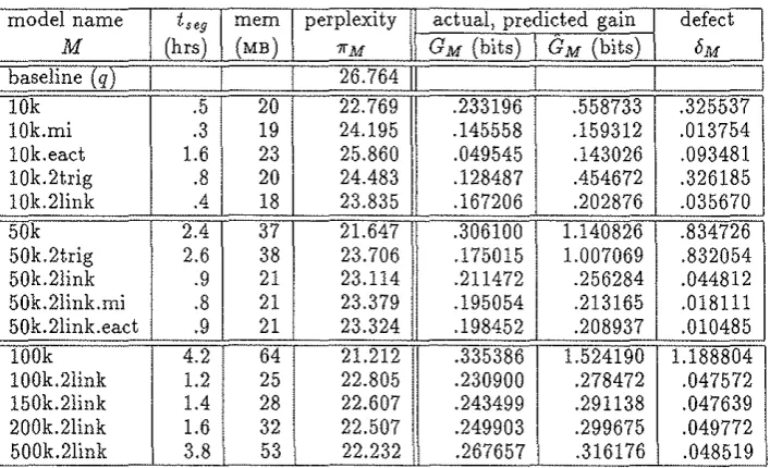
.01 before stopping. We write 1i'M for the perplexity of the final model M.

Table 2 summarizes our models, the characteristics of the training computation, and the model perplexities. Column tseg is the time to complete one improved iter-ative scaling iteration on one segment (!/40th) of the complete training corpus on an IBM RS/6000 POW-ERstation, model 590H. Column mem is the total data memory required to process one segment of the corpus. The columns for GM,

GM

and bM are discusseQ./below. We draw three conclusions from the perplexitY results in this table. First, models constructed only vyith 2link features have lower perplexity than those constructed only with 2trig features, when we compare models of the same size. This is evident in the comparison between 10k.2trig and 10k.2link, and also between 50k.2trig and 50k.2link. We believe this reflects the higher additivity of 2link gains, a point we discuss further in the next section. However, another possible explanation is that the training converges faster for 2link features than for 2trig features.

Second1 the best performance is obtained by

includ-ing both feature types. This can be seen by comparinclud-ing among models lOk, 10k.2trig and 10k.2link, and like-wise among 50k, 50k.2trig and 50k.2link.

Finally, models selected by gain do better than those selected by mutual information or empirical activa-tion. This is evident from the perplexities of mod-els lOk, lOk.mi and lOk.eact, and likewise 50k.2link, 50k.2link.rni and 50k.2link.eact.

Empirical Study of Gain Additivity

To investigate the additivity of the gainl we first com-puted the actual gain of each model M, defined as

1 PM(C)

GM

=

N log P(C) . (19)

Here PM(

C)

is the probability of the corpus, as given by model M. Note that the gain and the perplexity

are ~elated by GM

=

log(11',/11'M), where 11'q is the

per-plexity of the base model. We then compared G M with the gain as predicted by summing the individual feature gainsl written

GM"'

L

Gt. (20)

/EM

Table 2 reports both these values, and also their defect

OM, which is defined as OM

=

GM- GM. The defect measures the extent to which the model fails to realize its potential gain. The smaller the defect, the more nearly the gains of the underlying features are additive. We have argued that the additivity of the gain is related to the ¢-orthogonality of the feature set, and we believe this is borne out by the figures in the table. Trigger features are clearly highly non-additive. This is to be expectedl since in any collection of gainful trigger features1 we would expect a large fraction of them to

be potentially active at any one position.

By contrast1 the link features appear to be very

nearly additive. Moreover1 the defect OM does not grow monotonically with the number of link features in the model. It would seem that the stanza of 300,000 lower-ranked link features are more nearly ¢-orthogonal than the 2001000 higher-ranked ones. This is reasonable1 since on balance the lower-ranked features are probably less often active1 hence more likely to act independently

of one another.

Summary

In this paper we have investigated the use of gain as a criter.ion for selecting features for MEMD language mod-els. We showed how the gain of a feature arises natu-rally from consideration of the feature's predictive value in an MEMD model, compared to the predictions made by the base model. We argued that the gain is the prefered figure of merit for feature selection, since it identifies features that improve upon the base model.

We then applied this statistic to the problem of se-lecting features for a dependency grammar language model. We showed that when comparing models con-structed from the same number of features1 using gain

as the figure of merit yields models of lower perplexity than either empirical activation of mutual information. Moreover1 among models built exclusively from either

trigger or link features, but having the same number of features, those built exclusively from links had lower perplexity. However l we achieved the lowest perplex-ity when we picked the most gainful features without regard to their type.

model name

M

I

baseline (

q)

lOk lOk.mi lOk.eact 10k.2trig 10k.2link 50k 50k.2trig 50k.2link 50k.2link.mi 50k.2link.eact lOOk 100k.2link 150k.2link 200k.2link 500k.2link

.5 20 .3 19 1.6 23 .8 20 .4 18 2.4 37 2.6 38 .9 21 .8 21 .9 21 4.2 64 1.2 25 1.4 28 1.6 32 3.8 53

22.769 24.195 25.860 24.483 23.835 21.647 23.706 23.114 23.379 23.324 21.212 22.805 22.607 22.507 22.232

actual, predicted gain

GM (bits) GM (bits)

.233196 .558733 .145558 .159312 .049545 .143026 .128487 .454672 .167206 .202876 .306100 1.140826 .175015 1.007069 .211472 .256284 .195054 .213165 .198452 .208937

.335386 1.524190 .230900 .278472 .243499 .291138 .249903 .299675 .267657 .316176

.325537 .013754 .093481 .326185 .035670 .834726 .832054 .044812 .018111 .010485 1.188804 .047572 .047639 .049772 .048519

Table 2: Model Features, Training Characteristics, Perplexities, Gains. Models are named by the following convention. The first part of the name gives the number of features; the letter k denotes a factor of 1 ,000. Thus 10k is a model built of the 10,000 highest-ranking features of the candidate set F. The notation 2trig

or 2link means that we used only trigger or link features respectively. Thus 1 Ok.2link is built of the 10,000 highest-ranking 2link features of F. Additional letters identify the figure of merit used for the ranking: eact

stands for empirical activation, mi stands for mutual information. If neither appears, the figure of merit was the gain.

We hasten to point out that our results concern per-plexity only. It remains to be seen if these conclusions carry over to word error rate, in a suitable speech recog-nition experiment.

Acknowledgements

We gratefully acknowledge support in part by the Na-tional Science Foundation, grant IRI-9314969.

References

[1] D. Beeferman, A. Berger, J. Lafferty, "A Model of Lexical Attraction and Repulsion,'' Proc. of the ACL-EACL'97 Joint Conference, Madrid, Spain.

[2] A. Berger, S. Della Pietra, V. Della Pietra, "A Maximum Entropy Approach to Natural Language Processing,'' Computational Linguistics, 22(1): 39-71, March 1996.

[3] C. Chelba, et. al., "Structure and Performance of a Dependency Language Model," Proc. of Eu-rospeech '97, Rhodes, Greece, September 1997.

[4] S. Della Pietra, V. Della Pietra, J. Gillett, J. Laf-ferty, H. Printz, L. UreS, "Inference and Estima-tion of a Long-Range Trigram Model,)' Second In-ternational Colloquium on Grammatical Inference, Alicante, Spain, September 1994.

[5] S. Della Pietra, V. Della Pietra, and J. Lafferty, Inducing Features of Random Fields, IEEE

Trans-actions on Pattern Analysis and Machine Intelli-gence, 19(4): 380-393, April1997.

[6] R. Lau, R. Rosenfeld, S. Roukos, "Trigger-Based Language Models: a Maximum Entropy Ap-proach,'' Proc. of the International Conference on Acoustics, Speech and Signal Processing, pp II: 45-48, Minneapolis, MN, April 1993.

[7] D. Magerman, Natural Language Parsing as Sta-tistical Pattern Recognition, Ph.D. Thesis, Depart-ment of Computer Science, Stanford University, Palo Alto, CA, February 1994.

[8] H. Printz, "Fast Computation of Maximum En-tropy / Minimum Divergence Feature Gain," sub-mitted to International Conference on Speech and

Language Processing, Sydney, Australia, Septem-ber 1998.

[9] P. S. Rao, S. Dharanipragada, S. Roukos, "MDI Adaptation of Language Models Across Corpora," Proc. of Eurospeech '97, pages 1979-1982, Rhodes, Greece, September 1997.

[10] A. Ratnaparkhi, J. Reynar, S. Roukos, "A Maxi-mum Entropy Model for Prepositional Phrase At-tachment," Proc. of the Human Language Technol-ogy Workshop, Plainsboro, NJ, March 1994.

[image:10.594.122.476.72.287.2]