Exact Sampling and Decoding in High-Order Hidden Markov Models
Simon Carter∗
ISLA, University of Amsterdam Science Park 904, 1098 XH Amsterdam,
The Netherlands
Marc Dymetman Guillaume Bouchard
Xerox Research Centre Europe 6, chemin de Maupertuis
38240 Meylan, France
{first.last}@xrce.xerox.com
Abstract
We present a method for exact optimization and sampling from high order Hidden Markov Models (HMMs), which are generally han-dled by approximation techniques. Motivated by adaptive rejection sampling and heuris-tic search, we propose a strategy based on sequentially refining a lower-order language model that is an upper bound on the true model we wish to decode and sample from. This allows us to build tractable variable-order HMMs. The ARPA format for language mod-els is extended to enable an efficient use of the
max-backoff quantities required to compute the upper bound. We evaluate our approach on two problems: a SMS-retrieval task and a POS tagging experiment using 5-gram mod-els. Results show that the same approach can be used for exact optimization and sampling, while explicitly constructing only a fraction of the total implicit state-space.
1 Introduction
In NLP, sampling is important for many real tasks, such as: (i) diversity in language generation or machine translation (proposing multiple alternatives which are not clustered around a single maximum); (ii) Bayes error minimization, for instance in Statis-tical Machine Translation (Kumar and Byrne, 2004); (iii) learning of parametric and non-parametric Bayesian models (Teh, 2006).
However, most practical sampling algorithms are based on MCMC, i.e. they are based on local moves ∗This work was conducted during an internship at XRCE.
starting from an initial valid configuration. Often, these algorithms are stuck in local minima, i.e. in a basin of attraction close to the initialization, and the method does not really sample the whole state space. This is a problem when there are ambiguities in the distribution we want to sample from: by hav-ing a local approach such as MCMC, we might only explore states that are close to a given configuration. The necessity of exact sampling can be ques-tioned in practice. Approximate sampling tech-niques have been developed over the last century and seem sufficient for most purposes. However, the cases where one actually knows the quality of a sampling algorithm are very rare, and it is com-mon practice to forget about the approximation and simply treat the result of a sampler as a set of i.i.d. data. Exact sampling provides a de-facto guarantee that the samples are truly independent. This is par-ticularly relevant when one uses a cascade of algo-rithms in complex NLP processing chains, as shown by (Finkel et al., 2006) in their work on linguistic annotation pipelines.
In this paper, we present an approach for exact decoding and sampling with an HMM whose hid-den layer is a high-order language model (LM), which innovates on existing techniques in the fol-lowing ways. First, it is a joint approach to sam-pling and optimization (i.e. decoding), which is based on introducing a simplified, “optimistic”, ver-sion q(x) of the underlying language model p(x),
for which it is tractable to use standard dynamic pro-gramming techniques both for sampling and opti-mization. We then formulate the problem of sam-pling/optimization with the original model p(x) in
terms of a novel algorithm which can be viewed as a form of adaptive rejection sampling (Gilks and Wild, 1992; Gorur and Teh, 2008), in which a low acceptance rate (in sampling) or a low ratio p(x∗)/q(x∗) (in optimization, with x∗ the argmax ofq) leads to a refinement ofq, i.e., a slightly more complex and less optimisticq but with a higher ac-ceptance rate or ratio.
Second, it is the first technique that we are aware of which is able to performexact samplingwith such models. Known techniques for sampling in such situations have to rely on approximation techniques such as Gibbs or Beam sampling (see e.g. (Teh et al., 2006; Van Gael et al., 2008)). By contrast, our technique produces exact samples from the start, al-though in principle, the first sample may be obtained only after a long series of rejections (and therefore refinements). In practice, our experiments indicate that a good acceptance rate is obtained after a rel-atively small number of refinements. It should be noted that, in the case of exact optimization, a silar technique to ours has been proposed in an im-age processing context (Kam and Kopec, 1996), but without any connection to sampling. That paper, written in the context of image processing, appears to be little known in the NLP community.
Overall, our method is of particular interest be-cause it allows for exact decoding and sampling from HMMs where the applications of existing dy-namic programming algorithms such as Viterbi de-coding (Rabiner, 1989) or Forward-Backward sam-pling (Scott, 2002) are not feasible, due to a large state space.
In Section 2, we present our approach and describe our joint algorithm for HMM sam-pling/optimization, giving details about our exten-sion of the ARPA format and refinement proce-dure. In Section 3 we define our two experimental tasks, SMS-retrieval and POS tagging, for which we present the results of our joint algorithm. We finally discuss perspectives and conclude in Section 4.
2 Adaptive rejection sampling and heuristic search for high-order HMMs Notation Let x = {x1, x2, ...x�} be a given hid-den state sequence (e.g. eachxi is an English word) which takes values in X = {1,· · · , N}� where �
is the length of the sequence and N is the number of latent symbols. Subsequences(xa, xa+1,· · · , xb) are denoted by xba, where 1 ≤ a ≤ b ≤ �. Let o = {o1, o2, ...o�} be the set of observations asso-ciated to these words (e.g. oi is an acoustic realiza-tion of xi). The notations p, q and q� refer to un-normalized densities, i.e. non-negative measures on
X. Since only discrete spaces are considered, we
use for short p(x) = p({x}). When the context is not ambiguous, sampling according to p means sampling according to the distribution with density
¯
p(x) = pp((Xx)), wherep(X) = �Xp(x)dxis the total mass of the unnormalized distributionp.
Sampling The objective is to sample a se-quence with density p¯(x) proportional to p(x) =
plm(x)pobs(o|x) where plm is the probability of the sequence x under a n-gram model and pobs(o|x) is the probability of observing the noisy sequence o given that the correct/latent sequence is x. As-suming the observations depend only on the current state, this probability becomes
p(x) =
�
�
i=1
plm(xi|xii−−1n+1)pobs(oi|xi) . (1)
To find the most likely sequence given an ob-servation, or to sample sequences from Equa-tion 1, standard dynamic programming techniques are used (Rabiner, 1989; Scott, 2002) by expand-ing the state space at each position. However, as the transition ordernincreases, or the number of la-tent tokensN that can emit to each observationol increases, the dynamic programming approach be-comes intractable, as the number of operations in-creases exponentially in the order ofO(�Nn).
If one can find a proposal distributionqwhich is an upper bound ofp— i.e such thatq(x)≥p(x)for all sequencesx∈ X — and which it is easy to sam-ple from, the standardrejection samplingalgorithm can be used:
1. Samplex∼q/q(X), withq(X) =�X q(x)dx;
2. Accept x with probability p(x)/q(x),
other-wise rejectx;
!""#$%
&'(% !"#!$% )(*%!"%$&%
&+,% !"#'(% -#./,)%
!")*+,(%%
$% 0% 1% )(*4%!"%$&-% 2% 3%
(a)
!""#$%
$% &%
'()%
*)+%
*)+% !"#!$%
!%&$'(#!$%
!"&$'% #,-./*% '0/%
*)+1%!"&$')%
*)+1% !"&$')%
2% 3%
4%
5% !"#*+%
!",-./+&%
[image:3.612.80.540.41.106.2](b)
Figure 1: An example of an initialq-automaton (a), and the refinedq-automaton (b) Each state corresponds
to a context (only state 6 has a non-empty context) and each edge represents the emission of a symbol. Thick edges are representing the path for the sampling/decoding of two dog(s) barked, thin edges corresponding to alternative symbols. By construction,w1(dog)≥w2(dog|two)so that the total weight of (b) is smaller than the total weight of (a).
the average acceptance rate — which is equal to p(X)/q(X) — can be so large that rejection
sam-pling is not practical. Inadaptive rejection sampling
(ARS), the initial boundqis incrementally improved based on the values of the rejected elements. While often based on log-concave distributions which are easy to bound, ARS is valid for any type of bound, and in particular can be applied to the upper bounds onn-gram models introduced by (Kam and Kopec, 1996) in the context of optimization. When a sam-ple is rejected, our algorithm assumes that a small set of refined proposals is available, sayq�1,· · · , qm� , wheremis a small integer value. These refinements are improved versions of the current proposal q in the sense that they still upper-bound the target dis-tributionp, but their mass is strictly smaller than the mass ofq, i.e. q�(X) < q(X). Thus, each such
re-finement q�, while still being optimistic relative to the target distribution p, has higher average accep-tance rate than the previous upper boundq. A bound on then-gram LM will be presented in Section 2.1.
Optimization In the case of optimization, the ob-jective is to find the sequence maximizing p(x).
Viterbi on high-order HMMs is intractable but we have access to an upper bound q, for which Viterbi is tractable. Sampling from q is then replaced by finding the maximum pointxofq, looking at the ra-tior(x) =p(x)/q(x), and acceptingxif this ratio is equal to1, otherwise refiningq intoq� exactly as in the sampling case. This technique is able to find the exact maximum ofp, similarly to standard heuristic search algorithms based on optimistic bounds. We stop the process when q and p agree at the value maximizingq which implies that we have found the global maximum.
2.1 Upper bounds forn-gram models
To apply ARS on the target density given by Equation 1 we need to define a random se-quence of proposal distributions{q(t)}∞
t=1such that q(t)(x) ≥ p(x),∀x ∈ X,∀t ∈ {0,1,· · · }. Eachn-gramxi−n+1, ..., xi in the hidden layer con-tributes an n-th order factor wn(xi|xii−−1n+1) ≡ plm(xi|xii−−n1+1)pobs(oi|xi). The key idea is that these n-th order factors can be upper bounded by factors of ordern−kby maximizing over the head (i.e. prefix) of the context, as if part of the con-text was “forgotten”. Formally, we define the max-backoff weightsas:
wn−k(xi|xii−−1n+1+k)≡ max xii−−nn++1k
wn(xi|xii−−1n+1),
(2) By construction, the max-backoff weightswn−kare factors of ordern−kand can be used as surrogates to the original n-th order factors of Equation (1), leading to a nested sequence of upper bounds until reaching binary or unary factors:
p(x) = Π�i=1wn(xi|xii−−1n+1) (3)
≤ Π�i=1wn−1(xi|xii−−1n+2) (4)
· · ·
≤ Π�i=1w2(xi|xi−1) (5)
≤ Π�i=1w1(xi) :=q(0)(x) . (6) Now, one can see that the loosest bound (6) based on unigrams corresponds to a completely factorized distribution which is straightforward to sample and optimize. The bigram bound (5) corresponds to a standard HMM probability that can be efficiently de-coded (using Viterbi algorithm) and sampled (using backward filtering-forward sampling).1 In the con-text of ARS, our initial proposal q(0)(x) is set to 1Backward filtering-forward sampling (Scott, 2002) refers
the unigram bound (6). The bound is then incre-mentally improved by adaptively refining the max-backoff weights based on the values of the rejected samples. Here, a refinement refers to the increase of the order ofsomeof the max-backoff weights in the current proposal (thus most refinements consist ofn-grams with heterogeneous max-backoff orders, not only those shown in equations (3)-(6)). This operation tends to tighten the bound and therefore increase the acceptance probability of the rejection sampler, at the price of a higher sampling complex-ity. The are several possible ways of choosing the weights to refine; in Section 2.2 different refinement strategies will be discussed, but the main technical difficulty remains in the efficient exact optimization and sampling of a HMM with n-grams of variable orders. The construction of the refinement sequence
{q(t)}
t≥0 can be easily explained and implemented through a Weighted Finite State Automaton (WFSA) referred as aq-automaton, as illustrated in the fol-lowing example.
Example We give now a high-level description of the refinement process to give a better intuition of our method. In Fig. 1(a), we show a WFSA rep-resenting the initial proposal q(0) corresponding to an example with an acoustic realization of the se-quence of words (the,two,dogs,barked). The weights on edges of thisq-automaton correspond to the unigram max-backoffs, so that the total weight corresponds to Equation (6). Considering sampling, we suppose that the first sample fromq(0)produces
x1 = (the, two, dog, barked), marked
with bold edges in the drawing. Now, computing the ratio p(x1)/q(0)(x1) gives a result much below 1,
because from the viewpoint of the full modelp, the trigram(the two dog)is very unlikely; in other words the ratiow3(dog|the two)/w1(dog)(and,
in fact, already the ratio w2(dog|two)/w1(dog)) is very low. Thus, with high probability, x1 is jected. When this is the case, we produce a re-fined proposal q(1), represented by the WFSA in Fig. 1(b), which takes into account the more
real-1989), which creates a lattice of forward probabilities that con-tains the probability of ending in a latent state at a specific time
t, given the subsequence of previous observationsot
1, for all the
previous latent sub-sequencesxt1−1, and then recursively
mov-ing backwards, samplmov-ing a latent state based on these probabil-ities.
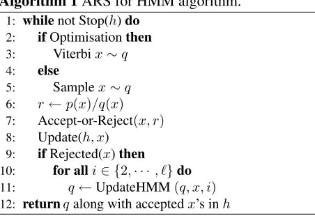
Algorithm 1ARS for HMM algorithm.
1: whilenot Stop(h)do
2: ifOptimisationthen
3: Viterbix∼q 4: else
5: Samplex∼q 6: r←p(x)/q(x)
7: Accept-or-Reject(x, r)
8: Update(h, x) 9: ifRejected(x)then
10: for alli∈ {2,· · ·, �}do
11: q←UpdateHMM(q, x, i)
12: returnqalong with acceptedx’s inh
Algorithm 2UpdateHMM
Input: A triplet(q, x, i)whereqis a WFSA,xis a
se-quence determining a unique path in the WFSA and iis a position at which a refinement must be done. 1: n:=ORDERi(xi1) + 1 #impliesxii−−1n+2∈Si−1
2: ifxii−−1n+1∈/ Si−1then
3: CREATE-STATE(xi−1
i−n+1, i−1)
4: #move incoming edges, keeping WFSA determin-istic
5: for alls∈SUFi−2(xii−−2n+1)do
6: e:=EDGE(s, xi−1)
7: MOVE-EDGE-END(e,xi−1 i−n+1)
8: #create outgoing edges
9: for all(s, l, ω)∈Ti(xii−−1n+2)do
10: CREATE-EDGE(xi−1
i−n+1,s,l,ω)
11: #update weights
12: for alls∈SUFi−1(xii−−1n+1)do
13: weight of EDGE(s, xi) :=wn(xi|xii−−1n+1)
14: return
istic weightw2(dog|two)by adding a node (node 6) for the contexttwo. We then perform a sampling trial withq(1), which this time tends to avoid produc-ingdog in the context oftwo; if the new sample is rejected, the refinement process continues until we start observing that the acceptance rate reaches a fixed threshold value. The case of optimization is similar. Suppose that withq(0) the maximum isx
1, then we observe thatp(x1) is lower thanq(0)(x1),
reject suboptimalx1 and refineq(0)intoq(1).
2.2 Algorithm
We describe in detail the algorithm and procedure for updating a q-automaton with a max-backoff of longer context.
[image:4.612.314.540.64.224.2]sam-pling/optimization strategy. On line 1, hrepresents the history of all trials so far, where the stopping cri-terion for decoding is whether the last trial in the history has been accepted, and for sampling whether the ratio of accepted trials relative to all trials ex-ceeds a certain threshold. The WFSA is initial-ized so that all transitions only take into account thew1(xi) max-backoffs, i.e. the initial optimistic-bound ignores all contexts. Then depending on whether we are sampling or decoding, in lines 2-5, we draw an event from our automaton using either the Viterbi algorithm or Forward-Backward sam-pling. If the sequence is rejected at line 7, then the q-automaton is updated in lines 10 and 11. This is done by expanding all the factors involved in the sampling/decoding of the rejected sequence x to a higher order. That is, while sampling or decoding the automaton using the current proposal q(t), the contexts used in the path of the rejected sequence are replaced with higher order contexts in the new refined proposalqt+1(x).
The update process of the q-automaton repre-sented as a WFSA is described in Algorithm 2. This procedure guarantees that a lower, more realistic weight is used in all paths containing the n-gram xii−n+1 while decoding/sampling the q-automaton, wherenis the order at whichxi
i−n+1 has been ex-panded so far. The algorithm takes as input a max-backoff function, and refines the WFSA such that any paths that include this n-gram have a smaller weight thanks to the fact that higher-order max-backoff have automatically smaller weights.
The algorithm requires the following functions:
• ORDERi(x) returns the order at which then -gram has been expanded so far at positioni.
• Sireturns the states at a positioni.
• Ti(s) returns end states, labels and weights of all edges that originate from this state.
• SUFi(x)returns the states atiwhich have a suf-fix matching the given context x. For empty contexts, all states atiare returned.
• EDGE(s, l) returns the edge which originates fromsand has label l. Deterministic WFSA, such as those used here, can only have a single transition with a labellleaving from a states.
• CREATE-STATE(s, i) creates a state with name s at position i, CREATE-EDGE(s1, s2, l, ω) creates an edge (s1, s2)
between s1 and s2 with weight ω and label l, and MOVE-EDGE-END(e, s) sets the end of edge e to be the state s, keeping the same starting state, weight and label.
At line 1, the expansion of the currentn-gram is increased by one so that we only need to expand con-texts of sizen−2. Line 2 checks whether the
con-text state exists. If it doesn’t it is created at lines 3-10. Finally, the weight of the edges that could be in-volved in the decoding of thisn-gram are updated to a smaller value given by a higher-order max-backoff weight.
The creation of a new state in lines 3-10 is straightforward: At lines 5-7, incoming edges are moved from states at positioni−2 with a
match-ing context to the newly created edge. At lines 9-10 edges heading out of the context state are cre-ated. They are simply copied over from all edges that originate from the suffix of the context state, as we know these will be legitimate transitions (i.e we will always transition to a state of the same order or lower).
Note that we can derive many other variants of Algorithm 2 which also guarantee a smaller total weight for theq-automaton. We chose to present this version because it is relatively simple to implement, and numerical experiments comparing different re-finement approaches (including replacing the max-backoffs with the highest-possible context, or pick-ing a spick-ingle “culprit” to refine) showed that this ap-proach gives a good trade-off between model com-plexity and running time.
2.3 Computing Max-Backoff Factors
An interesting property of the max-backoff weights is that they can be computed recursively; taking a 3-gram LM as an example, we have:
w1(xi) = max xi−1
w2(xi|xi−1)
w2(xi|xi−1) = max xi−2
w3(xi|xii−−12)
w3(xi|xii−−12) = p(xi|xii−−12)p(oi|xi).
conditional probability of the observation), as any extra context is discarded by the 3-gram language model. It’s easy to see that as we refine q(t) by replacing existing max-backoff weights with more specific contexts, theq(t)tends topatttends to in-finity.
In the HMM formulation, we need to be able to efficiently compute at run-time the max-backoffs w1(the), w2(dog|the), · · ·, taking into account smoothing. To do so, we present a novel method for converting language models in the standard ARPA format used by common toolkits such as (Stolcke, 2002) into a format that we can use. The ARPA file format is a tableT composed of three columns: (1) an n-gram which has been observed in the training corpus, (2) the log of the conditional probability of the last word in then-gram given the previous words (log f(.)), and (3) a backoff weight (bow(.)) used when unseenn−grams ’backoff’ to thisn-gram.2
The probability of any n-gramxii−n (in the pre-vious sense, i.e. writingp(xii−n)forp(xi|xii−−1n)) is then computed recursively as:
p(xii−n) =
�
f(xii−n) ifxii−n∈T bow(xii−−1n)p(xii−n+1) otherwise.
(7) Here, it is understood that if xii−−1n is in T, then its bow(.) is read from the table, otherwise it is taken to be 1.
Different smoothing techniques will lead to dif-ferent calculations of f(xii−n)and bow(xii−−1n),
how-ever both backoff and linear-interpolation methods can be formulated using the above equation.
Starting from the ARPA format, we pre-compute a new table MAX-ARPA, which has the same lines as ARPA, each corresponding to ann-gramxi
i−n ob-served in the corpus, and the same f and bow, but with two additional columns: (4) a max log prob-ability (log mf(xi
i−n)), which is equal to the maxi-mum log probability over all then-grams extending the context ofxii−n, i.e. which havexii−nas a suffix; (5) a “max backoff” weight (mbow(xi
i−n)), which is a number used for computing the max log probabil-ity of an n-gram not listed in the table. From the MAX-ARPA table, the max probabilitywof anyn
-2See www.speech.sri.com/projects/srilm/
manpages/ngram-format.5.html, last accessed at
1/3/2012, for further details.
gramxii−n, i.e the maximum ofp(xii−n−k)over all
n-grams extending the context ofxi
i−n, can then be computed recursively (again very quickly) as:
w(xii−n) =
�
mf(xii−n) ifxii−n∈T mbow(xii−−1n)p(xii−n) otherwise.
(8) Here, if xii−−1n is in T, then its mbow(.) is read from the table, otherwise it is taken to be 1. Also note that the procedure callsp, which is computed as described in Equation 7.3
3 Experiments
In this section we empirically evaluate our joint, ex-act decoder and sampler on two tasks; SMS-retrieval (Section 3.1), and supervised POS tagging (Sec-tion 3.2).
3.1 SMS-Retrieval
We evaluate our approach on an SMS-message re-trieval task. A latent variable x ∈ {1,· · · , N}� represents a sentence represented as a sequence of words: N is the number of possible words in the vocabulary and � is the number of words in the sentence. Each word is converted into a sequence of numbers based on a mobile phone numeric key-pad. The standard character-to-numeric function num : {a,b,· · ·,z, .,· · ·,?}→{1,2,· · ·,9,0} is used. For example, the words dog and fog
are represented by the sequence (3,6,4) because
num(d)=num(f)=3, num(o)=6 and num(g)=4. Hence, observed sequences are sequences of nu-meric strings separated by white spaces. To take into account typing errors, we assume we observe a noisy version of the correct numeric sequence
(num(xi1),· · · ,num(xi|xi|) that encodes the word
xi at thei-th position of the sentencex. The noise model is:
p(oi|xi)∝
|xi| �
t=1
1
k∗d(oit,num(xit)) + 1
, (9)
where d(a, b) is the physical distance between the
numeric keysaandbandkis a user provided con-3In this discussion of the MAX-ARPA table we have ignored
0 10 20 30 40 50 60 70 80 90 100
1 2 3 4 5 6 7 8 9 10
avg #iterations
input length
3 4 5
0 50 100 150 200 250 300 350 400 450 500
1 2 3 4 5 6 7 8 9 10
avg #states
input length
[image:7.612.72.301.71.149.2]3 4 5
Figure 2: On the left we report the average # of iterations taken to decode given different LMs over input sentences of different lengths, and on the right we show the average # of states in the finalq
-automaton once decoding is completed.
stant that controls the ambiguity in the distribution; we use 64 to obtain moderately noisy sequences.
We used the English side of the Europarl cor-pus (Koehn, 2005). The language model was trained using SRILM (Stolcke, 2002) on 90% of the sen-tences. On the remaining 10%, we randomly se-lected 100 sequences for lengths 1 to 10 to obtain 1000 sequences from which we removed the ones containing numbers, obtaining a test set of size 926.
Decoding Algorithm 1 was run in the optimization mode. In the left plot of Fig. 2, we show the number of iterations (running Viterbi then updating q) that the differentn-gram models of size 3, 4 and 5 take to do exact decoding of the test-set. For a fixed sen-tence length, we can see that decoding with larger n-gram models leads to a sub-linear increase w.r.t. nin the number of iterations taken. In the right plot of Fig. 2, we show the average number of states in our variable-order HMMs.
To demonstrate the reduced nature of our q -automaton, we show in Tab. 1 the distribution of n-grams in our final model for a specific input sen-tence of length 10. The number ofn-grams in the full model is∼3.0×10¹⁵. Exact decoding here is not tractable using existing techniques. Our HMM has only 9008n-grams in total, including 118 5-grams.
n: 1 2 3 4 5
q: 7868 615 231 176 118
Table 1: # ofn-grams in our variable-order HMM.
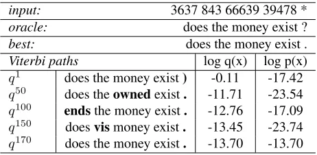
Finally, we show in Tab. 2 an example run of our algorithm in the optimization setting for a given
input. Note that the weight according to our q -automaton for the first path returned by the Viterbi algorithm is high in comparison to the true log prob-ability according top.
Sampling For the sampling experiments, we limit the number of latent tokens to 100. We refine ourq -automaton until we reach a certain fixed cumulative acceptance rate (AR). We also compute a rate based only on the last 100 trials (AR-100), as this tends to better reflect the current acceptance rate.
In Fig. 3a, we plot a running average of the ratio at each iteration over the last 10 trials, for a single sampling run using a 5-gram model for an example input. The ratios start off at10−20, but gradually
in-crease as we refine our HMM. After ∼ 500 trials, we start accepting samples fromp. In Fig. 3b, we show the respective ARs (bottom and top curves re-spectively), and the cumulative # of accepts (middle curve), for the same input. Because the cumulative accept ratio takes into account all trials, the final AR of 17.7% is an underestimate of the true accept ra-tio at the final iterara-tion; this final accept rara-tio can be better estimated on the basis of the last 100 trials, for which we read AR-100 to be at around 60%.
We note that there is a trade-off between the time needed to construct the forward probability lattice needed for sampling, and the time it takes to adapt the variable-order HMM. To resolve this, we pro-pose to use batch-updates: makingBtrials from the sameq-automaton, and then updating our model in one step. By doing this, we noted significant speed-ups in sampling times. In Tab. 3, we show various
input: 3637 843 66639 39478 *
oracle: does the money exist ?
best: does the money exist .
Viterbi paths log q(x) log p(x)
q1 does the money exist) -0.11 -17.42
q50 does theownedexist. -11.71 -23.54
q100 endsthe money exist. -12.76 -17.09
q150 doesvismoney exist. -13.45 -23.74
q170 does the money exist. -13.70 -13.70
Table 2: Viterbi paths given differentqt. Here, for
the given input, it took 170 iterations to find the best sequence according top, so we only show every 50th
[image:7.612.313.544.529.642.2]1e-20 1e-18 1e-16 1e-14 1e-12 1e-10 1e-08 1e-06 0.0001 0.01 1
0 500 1000 1500 2000
ratio
iterations
(a)
0 10 20 30 40 50 60
0 500 1000 1500 2000 0 100 200 300 400 500 600
accept ratio % # accepts
iterations #ACC
AR AR 100
(b)
100 200 300 400 500 600 700 800
1 2 3 4 5 6 7 8 9 10
avg #iterations
input length 5 4 3
(c)
0 200 400 600 800 1000 1200 1400 1600 1800
1 2 3 4 5 6 7 8 9 10
avg #states
input length 5
4 3
(d)
Figure 3:In 3a, we plot the running average over the last 10 trials of the ratio. In 3b, we plot the cumulative # of accepts (middle curve), the accept rate (bottom curve), and the accept rate based on the last 100 samples (top curve). In 3c, we plot the average number of iterations needed to sample up to an AR of 20% for sentences of different lengths in our test set, and in 3d, we show the average number of states in our HMMs for the same experiment.
B: 1 10 20 30 40 50 100
[image:8.612.72.525.41.138.2]time: 97.5 19.9 15.0 13.9 12.8 12.5 11.4 iter: 453 456 480 516 536 568 700
Table 3: In this table we show the average amount of time in seconds and the average number of iterations (iter) taken to sample sentences of length 10 given different values ofB.
statistics for sampling up to AR-100=20 given
dif-ferent values for B. We ran this experiment using the set of sentences of length 10. A value of 1 means that we refine our automaton after each rejected trial, a value of 10 means we wait until rejecting 10 trials before updating our automaton in one step. We can see that while higher values ofB lead to more iter-ations, as we do not need to re-compute the forward trellis needed for sampling, the time needed to reach the specific AR threshold actually decreases, from 97.5 seconds to 11.4 seconds, an 8.5% speedup. Un-less explicitly stated otherwise, further experiments use aB = 100.
We now present the full sampling results on our test-set in Fig. 3c and 3d, where we show the aver-age number of iterations and states in the final mod-els once refinements are finished (AR-100=20%) for different orders n over different lengths. We note a sub-linear increase in the average number of tri-als and states when moving to higher n; thus, for length=10, and forn = 3,4,5, # trials: 3-658.16,
4-683.3, 5-700.9, and # states: 3-1139.5, 4-1494.0, 5-1718.3.
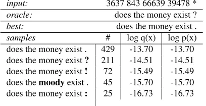
Finally, we show in Tab. 4, the ranked samples drawn from an input sentence, according to a 5-gram LM. After refining our model up to AR-100=20%,
input: 3637 843 66639 39478 * oracle: does the money exist ? best: does the money exist . samples # log q(x) log p(x) does the money exist . 429 -13.70 -13.70 does the money exist? 211 -14.51 -14.51 does the money exist! 72 -15.49 -15.49 does themoodyexist . 45 -15.70 -15.70 does the money exist: 25 -16.73 -16.73
Table 4: Top-5 ranked samples for an example in-put. We highlight in bold the words which are differ-ent to the Viterbi best of the model. The oracle and best are not the same for this input.
we continued drawing samples until we had 1000 exact samples from p (out of ∼ 4.7k trials). We show the count of each sequence in the 1000 sam-ples, and the log probability according topfor that event. We only present the top-five samples, though in total there were 90 unique sequences sampled, 50 of which were only sampled once.
3.2 POS-tagging
[image:8.612.326.530.238.343.2]95.6 95.65 95.7 95.75 95.8 95.85 95.9 95.95
3 4 5 6 7 8 9
accuracy %
n-gram order
(a)
0 2000 4000 6000 8000 10000 12000 14000 16000 18000
3 4 5 6 7 8 9
time
n-gram order ARS
F
(b)
50 60 70 80 90 100 110 120 130
3 4 5 6 7 8 9
avg #iterations
n-gram order
(c)
100 200 300 400 500 600 700 800 900
3 4 5 6 7 8 9
avg #states
[image:9.612.73.522.40.139.2]n-gram order (d)
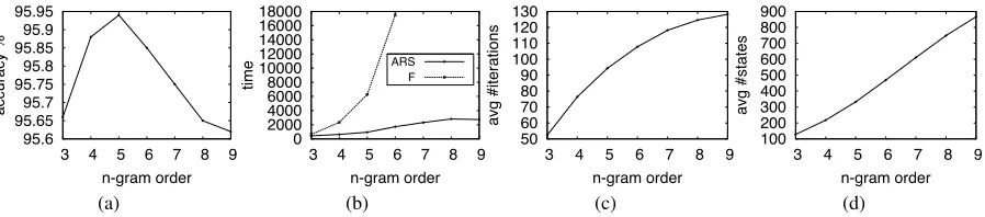
Figure 4: In 4a, we report the accuracy results given differentn-gram models on the WSJ test-set. In 4b, we
show the time taken (seconds) to decode the WSJ test-set given our method (ARS), and compare this to the full model (F). In 4c, the average number of iterations needed to sample the test-set given differentn-gram
language models is given, and 4d shows the average number of states in the variable-order HMMs.
sections 22-24.
We first present results for our decoding experi-ments. In Fig. 4a we show the accuracy results of our different models on the WSJ test-set. We see that the best result is achieved with the 5-gram LM giving an accuracy of 95.94%. After that, results start to drop, most likely due to over-fitting of the LM during training and an inability for the smooth-ing technique to correctly handle this.
In Fig. 4b, we compare the time it takes in seconds to decode the test-set with the full model at eachn -gram size; that is a WFSA with all context states and weights representing the true language model log probabilities. We can see that while increas-ing then-gram model size, our method (ARS) ex-hibits a linear increase in decoding time, in contrast to the exponential factor exhibited when running the Viterbi algorithm over the full WFSA (F). Note for n-gram models of order 7 and higher, we could not decode the entire test set as creating the full WFSA was taking too long.
Finally in both Figs 4c and 4d, we show the aver-age number of iterations taken to sample from the entire test-test, and the average number of states in our variable-order HMMs, with AR-100=60%.
Again we note a linear increase in both Fig., in con-trast to the exponential nature of standard techniques applied to the full HMM.
4 Conclusion and Perspectives
We have presented a dual-purpose algorithm that can be used for performing exact decoding and sampling on high-order HMMs. We demonstrated the valid-ity of our method on SMS-retrieval and POS exam-ples, showing that the “proposals” that we obtain
re-quire only a fraction of the space that would result from explicitly representing the HMM. We believe that this ability to support exact inference (both ap-proximation and sampling) at a reasonable cost has important applications, in particular when moving from inference to learning tasks, which we see as a natural extension of this work.
By proposing a common framework for sampling and optimization our approach has the advantage that we do not need separate skills or expertise to solve the two problems. In several situations, we might be interested not only in the most probable se-quence, but also in the distribution of the sequences, especially when diversity is important or in the pres-ence of underlying ambiguities.
2011) and hierarchical (Rush and Collins, 2011)) among others. However, sampling such distributions remains a difficult problem. We are currently ex-tending the approach described in this paper to han-dle such applications. Again, using ARS on a se-quence of upper bounds to the target distribution, our idea is to express one of the two models as a con-text free grammar and incrementally compute the intersection with the second model, maintaining a good trade-off between computational tractability of the refinement and a reasonable acceptance rate.
References
Thorsten Brants. 2001. Tnt - a statistical part-of-speech tagger. In Proceedings of the Sixth conference of Applied Natural Language Processing (ANLP 2001), pages 224–231.
Yin-Wen Chang and Michael Collins. 2011. Exact de-coding of phrase-based translation models through la-grangian relaxation. InProceedings of the Conference on Empirical Methods for Natural Language Process-ing (EMNLP 2011).
Jenny Rose Finkel, Christopher D. Manning, and An-drew Y. Ng. 2006. Solving the problem of cascading errors: approximate bayesian inference for linguistic annotation pipelines. In Proceedings of the Confer-ence on Empirical Methods in Natural Language Pro-cessing (EMNLP 2006), pages 618–626.
W. R. Gilks and P. Wild. 1992. Adaptive rejec-tion sampling for gibbs sampling. Applied Statistics, 42(2):337–348.
Dilan Gorur and Yee Whye Teh. 2008. Concave convex adaptive rejection sampling. Technical report, Gatsby Computational Neuroscience Unit.
Anthony C. Kam and Gary E. Kopec. 1996. Document image decoding by heuristic search. IEEE Transac-tions on Pattern Analysis and Machine Intelligence, 18:945–950.
Philipp Koehn. 2005. Europarl: A parallel corpus for statistical machine translation. InProceedings of Ma-chine Translation Summit (MT-Summit 2005), pages 79–86.
Shankar Kumar and William Byrne. 2004. Minimum bayes risk decoding for statistical machine translation. InJoint Conference of Human Language Technologies and the North American chapter of the Association for Computational Linguistics (HLT-NAACL 2004). Mitchell P. Marcus, Beatrice Santorini, and Mary Ann
Marcinkiewicz. 1993. Building a large annotated cor-pus of english: the penn treebank. Computional Lin-guistics, 19:313–330.
Lawrence R. Rabiner. 1989. A tutorial on hidden markov models and selected applications in speech recogni-tion. Proceedings of the IEEE, 77(2):257–286, Febru-ary.
Alexander M. Rush and Michael Collins. 2011. Exact decoding of syntactic translation models through la-grangian relaxation. InProceedings of the Conference on Empirical Methods for Natural Language Process-ing (EMNLP 2011), pages 26–37.
Alexander M. Rush, David Sontag, Michael Collins, and Tommi Jaakkola. 2010. On dual decomposition and linear programming relaxations for natural language processing. In Proceedings of the Conference on Empirical Methods for Natural Language Processing (EMNLP 2010).
Steven L. Scott. 2002. Bayesian methods for hidden markov models: Recursive computing in the 21st cen-tury. Journal of the American Statistical Association, 97:337–351.
Andreas Stolcke. 2002. Srilm - an extensible language modeling toolkit. InProceedings of the International Conference of Spoken Language Processing (INTER-SPEECH 2002), pages 257–286.
Yee Whye Teh, Michael I. Jordan, Matthew J. Beal, and David M. Blei. 2006. Hierarchical dirichlet pro-cesses. Journal of the American Statistical Associa-tion, 101(476):1566–1581.
Yee Whye Teh. 2006. A hierarchical bayesian language model based on pitman-yor processes. InProceedings of the 21st International Conference on Computational Linguistics and the 44th annual meeting of the As-sociation for Computational Linguistics (ACL 2006), pages 985–992.