Mustansar Ali Ghazanfar and Adam Prugel-Bennett
Abstract—A coalition is a set of self-interested agents that agree to cooperate for achieving a set of goals. Coalition formation is an active area of research in multi-agent systems nowadays. Central to this endeavour is the problem of determining which of the many possible coalitions to form in order to achieve some goal, which is called coalition structure generation. Coalition structure generation problem is extremely challenging due to the number of possible solutions that need to be examined, which grows exponentially with the number of agents involved. Generally, agents would enumerate all possible coalitions, store them in memory, and then try to construct the coalition structure that maximizes the sum of the values of the coalitions. However, this is not feasible when we have a large number of agents, and other constraints on execution time, and memory. Hence, there is a need to develop an algorithm that can generate solutions rapidly for large number of agents while can provide bounds on the value of solution as well. With this in mind, we propose two new heuristics, namely LocalSearch and GreedySearch, for generating the coalition structure, which satisfy these properties. We empirically show that these heuristics are able to return ‘good-enough’ solutions in very short time. They enhance the performance of state of the art algorithm, IP (proposed by [12]) in terms of increased lower bound, anytime property, and solution quality. Furthermore, we implemented different heuristics for selecting a sub-space in the IP algorithm and show how the time required to find a good-enough solution depends on the selection of a sub-space in the IP algorithm.
Index Terms—Multi-agent systems, Coalition formation, Coalition structure generation, Heuristics
I. INTRODUCTION
Cooperation among agents is an important keystone in Multi-Agent Systems (MAS), which enables them to solve a problem efficiently. Agents cooperate in many economic milieus on issues of common interest, which results in the formation of coalition [1]. For this purpose, agents need to determine the optimal set of agents with whom to enter into a coalition (i.e. the best grouping of agents). This problem is formally referred to as the Coalition Structure Generation (CSG) problem.
Suppose that we are given set of agents 1,2, … … 𝑛 𝜖 𝐴, and the value of a coalition , s, is specified by a characteristic function v(.). Then the value of the coalition structure (CS) is:
𝑉 𝐶𝑆 = (𝑣𝑠)
𝑆 𝜖 𝐶𝑆
Generally, the goal is to maximize the social welfare by discovering the optimal coalition structure [2].
CS* = arg 𝑚𝑎𝑥𝑆∈𝐶𝑆 𝑉(𝐶𝑆)
Finding the optimal coalition structure is very challenging as the computational complexity of finding the optimal coalition structure is exponential1 in the number of agents and is shown to beNP-hard [3]. To date, a number of algorithms have been proposed to solve CSG problem, but there has been less work on algorithms that can generate good-enough solutions quickly. In this paper, we propose new heuristics to solve this problem and show how good-enough solution can be generated, while balancing the properties, such as execution time and memory.
II. RELATED WORK
Existing literature defines various CSG algorithms that can be classified into three main classes: Dynamic Programming (DP) based algorithms, heuristic based algorithms, and anytime algorithms [4]. Dynamic programming algorithms generate optimal solution (i.e. optimal coalition structure) with minimal computational complexity. They provide a guarantee on the performance of the algorithm in the worst-case scenarios. [5], [6], [7] develop DP based algorithms but these algorithms can not be used for large number of agents (>20). Heuristic based algorithms are not designed to find the optimal solution; rather their focus is on finding good solutions. In this context, [8] employ an order-based genetic algorithm (OBGA) as a stochastic search process to discover the optimal coalition structure. The main limitation of this algorithm is that, it provides no guarantee about finding the optimal CS, and it
1
The number of coalition structure grows in O(𝑛𝑛) with the number
of agents [3].
Novel Heuristics for Coalition Structure
Generation in Multi-agent Systems
cannot specify any bounds on the quality of the optimal CS.
[9] developed a greedy algorithm, which takes only coalitions up to a certain size into consideration. Its limitation is that it provides no guarantee on the quality of its solutions compared to the actual optimal. Anytime algorithms return an initial solution, and then improve on the quality (and establish better bound gradually) of the solution as they search more of the space. In this context, [3] proposed an anytime algorithm that can establish a bound on quality of the solution, however, the algorithm has to search entire search space, to generate a guaranteed optimal solution2 and the bounds provided by the algorithm are not valuable for practical use. Based on this concept, [10] proposed another anytime algorithm that can also establish a bound on the quality of solution but employ different searching mechanism and have the same demerits. [11, 12] proposed a state of the art anytime algorithm, IP, but again it has to search entire space in order to generate an optimal solution.
III. BACKGROUND: INTEGER PARTITION GRAPH AND IP ALGORITHM
In [12] the authors proposed an efficient search space representation that can be used for finding the optimal solution efficiently. They called this representation Integer Partition Graph. In this representation, they partitioned the search space
𝑝 by defining sub-spaces that contain coalition structures that are similar according to the ‗integer partitions‘3 of the number of agents. This can be defined by a function 𝐹: 𝖕G , where
G is the set of integer partition of n. Then they defined a pre-image (or inverse pre-image) of an integer partition G as follows:
𝑃𝐺 = 𝐹−1 𝐺 .
Each pre-image, which represents a sub-space in the integer partition graph, encloses all the coalition structures corresponding to the same integer partition G.
Fig. 1 shows an integer partition graph for 4 agents. We observe that sub-spaces have been categorized into levels, based on the number of parts within the integer partitions. In general, we have n levels, where n is the number of agents. Each level, 𝖕𝑖 comprises of all the sub-spaces that correspond to an integer partition with 𝑖 parts.
Given this representation, they computed the Upper Bound4 (UB) and Lower Bound5 (LB) in each sub-space 𝑃𝐺 as follows: Let 𝐿𝑠 be the list of coalitions of size s, and let
2 i.e. bound=1
3
Integer partition of n is a multiset of positive integers that add up to exactly n.
4
UB places an upper limit on the value of the optimal solution, i.e. no coalition structure in a sub-space can have value greater than its UB.
[image:2.612.322.529.52.234.2]5 LB places a lower limit on the value of the optimal solution, i.e. the solution at worse will be greater than or equal to this LB.
Fig. 1: Example of the integer partition graph for 4 agents [12].
𝑚𝑎𝑥𝑠 , 𝑚𝑖𝑛𝑠 and 𝑎𝑣𝑔𝑠 be the maximum, minimum, and
average value of the coalition in 𝐿𝑠 respectively.
Now given an integer partition G, let 𝑇𝐺 be the Cartesian product of the lists 𝐿𝑠 : 𝑠 𝜖 𝐺, i.e.
𝑇𝐺 = (𝐿𝑠 )𝐺(𝑠)
𝑠 𝜖 𝐺
,
where G(s) is the multiplicity of s in G.
Now consider the value 𝑀𝐴𝑋𝐺 obtained by adding the maximum value of each element (i.e. coalition list) in 𝑇𝐺 . Formally, it can be represented as follows:
𝑀𝐴𝑋𝐺 = 𝑠 𝜖 𝐺𝑚𝑎𝑥𝑠 × G(s) .
This value is an upper bound on the best coalition structure in 𝑃𝐺 . Now the average value of all the solutions in 𝑃𝐺 , denoted by 𝐴𝑉𝐺𝐺 , can be computed immediately after scanning the input, by adding the averages of the coalition lists in 𝑃𝐺 . If we consider G= 𝑔1, 𝑔2,… , 𝑔|𝐺| as an integer partition, and 𝑎𝑣𝑔𝑔𝑖 as the average of the values of all coalition in 𝐿𝑔𝑖, then it can be computed as follows6:
𝐴𝑉𝐺𝐺 = 𝐺𝑖=1𝑎𝑣𝑔𝑔𝑖 .
Furthermore, they argued that it is better to specify 𝐴𝑉𝐺𝐺 as lower bound. The reason behind this is that one can prune a lot of search space by improving the LB7 and average value of a sub-space is usually better than the minimum value.
Two main steps that IP requires in order to search the space using this representation are,
a. Scanning the input in order to compute the bounds (i.e.
𝑀𝐴𝑋𝐺 and 𝐴𝑉𝐺𝐺 ) for every subspace 𝑃𝐺 .
6
For proof of this theorem, refer to [12]. 7
b. Selecting and searching within the remaining sub-spaces—we can apply different selection functions within this step (discussed in next section).
To get the unbiased performance evaluation of IP with other state of the art algorithms, they tested it under different distributions. They used the normal, uniform, and NDCS8 (Normally Distributed Coalition Structures) input distribution, and benchmarked it against the other state-of-the-art algorithm IDP. The results are shown in fig. 2.
Fig. 2: The time required to find the optimal solution for IDP and IP under NDCS, Normal, and Uniform Distributions [12]. IDP was found to be 15 times slower than IP.
They showed that IP was faster than IDP in finding the optimal coalition structure. Furthermore, they noted that IP was slower in finding the solution in the case of NDCS9.
IV. PROPOSED HEURISTICS
A. LocalSearch Heuristic
We assume that the input to coalition structure generation algorithm is the value associated to each coalition, v(C), where C 𝜖2𝐴/{𝜙}. We further assume that input is given as follows: C 𝐿𝑠 ∀𝑠 𝜖 {1,2, … . . 𝑛} and v 𝐿𝑠 ∀𝑠 𝜖 {1,2, … . . 𝑛}, where C 𝐿𝑠 is a list containing the coalitions and v 𝐿𝑠 is a list containing the values of all the coalitions of size s.
Now we define some notations. Let max (𝑣 (𝐿𝑠)) be the maximum value present in a list of value 𝑣(𝐿𝑠). Let MAX consists of memory locations10, that contain the maximum values (i.e. max (𝑣 (𝐿𝑠))) from each list of values present in G. Furthermore, let 𝑉𝑀𝑎𝑥 be the maximum value present in MAX
8 See appendix A.
9
Our heuristics are more successful in this case.
10 Its size is equal to the size of corresponding integer partition that we want to search, i.e., |MAX|= |G|.
(i.e. 𝑉𝑀𝑎𝑥 = max(𝑀𝐴𝑋)), 𝐿𝑀𝑎𝑥 be the list of coalition that contains this value 𝑉𝑀𝑎𝑥, and 𝐶𝑀𝑎𝑥 be the coalition that corresponds to the value 𝑉𝑀𝑎𝑥.
Like IP algorithm we first scan the value of coalition of size n (called grand coalition), scan the values of coalitions of size 1 (called singleton coalition), and search the level 2 (i.e. 𝔭2). At this point, we can compute the best solution found so for. Then we run LocalSearch heuristic that computes a good-enough solution.
The pseudo code of the LocalSearch heuristic can be outlined as follows:
Algorithm: LocalSearch()—Scans input, generates CS, and improves the LB of IP.
Input: C 𝑳𝒔 ∀𝒔 𝝐 {𝟏, 𝟐, … . . 𝒏}, v 𝑳𝒔 ∀𝒔 𝝐 {𝟏, 𝟐, … . . 𝒏}, set of
agents (A = 𝒂𝟏, … , 𝒂𝒏 ), an integer partition (G= 𝒈𝟏, 𝒈𝟐,… , 𝒈|𝑮|).
Output: coalition structure, value of the coalition structure, time required to generate the coalition structure.
1. Set solution= ―‖, value=0
2. end= |G| // Size of G
3. t1=start timer;
//Loop until we finish finding a valid solution. In each iteration, we pick the maximum possible coalition value from all available coalitions in that sub-space
4. While (end>=1)
//From step 5 to 7 we load lists into memory, pick maximum value of each list, and store these maximum values in an array MAX
5. Get lists of coalitions, C 𝑳𝑮 , from A
6. Get lists of values, v 𝑳𝑮 , corresponding to C 𝑳𝑮
7. Get the maximum value present in each list of value and store
them in an array MAX, i.e. MAX= [max (𝒗(𝑳𝒈𝟏)),
max(𝒗(𝑳𝒈𝟐),….. max (𝒗(𝑳𝒈|𝑮|))] //pick maximum value from
each list of values in G
//From step 8 to 10, we find the maximum value 𝑽𝑴𝒂𝒙, from MAX array and pick the coalition 𝑪𝑴𝒂𝒙 which corresponds to this value
8. Get element, 𝑽𝑴𝒂𝒙, which has the maximum value in MAX,
i.e. 𝑽𝑴𝒂𝒙= max(MAX)
9. Find index of 𝑽𝑴𝒂𝒙 in MAX and find corresponding list, 𝑳𝑴𝒂𝒙
from G, which contains this element 𝑽𝑴𝒂𝒙 //find out the list
which contains this maximum value, 𝑽𝑴𝒂𝒙
10. Search for the coalition, 𝑪𝑴𝒂𝒙, which has value 𝑽𝑴𝒂𝒙, in
corresponding list 𝑳𝑴𝒂𝒙
//In step 11 and 12, we add 𝑽𝑴𝒂𝒙 and 𝑪𝑴𝒂𝒙 in solution value and solution respectively
11. Value = value+ 𝑽𝑴𝒂𝒙 //add coalition value
12. Solution = solution + 𝑪𝑴𝒂𝒙 //add coalition
// From step 13 to 17, we update (except in last iteration) MAX, G, and A
13. If !(end ==1)
14. Update MAX: set all element of MAX to zero,
and set |MAX|= |MAX| -1
15. Update G: delete 𝑳𝑴𝒂𝒙from G, and set |G| = |G| -1
[image:3.612.57.296.186.379.2]17. End if
18. end =end -1; //update loop counter
19. End while
20. t2=stop timer;
21. Return (solution, value, t2-t1)
At start, we pick up the integer partition G, and load its list of coalitions and values in memory (step 5 and 6). Then we find the maximum value from each list and store these values in an array, MAX (step 7). Now we find the maximum value, 𝑉𝑀𝑎𝑥, from this array and get the coalition list, 𝑳𝑀𝑎𝑥 ,that contains this value. From this list, we find the coalition, 𝑪𝑀𝑎𝑥 that corresponds to this maximum value (step 8 to 10). Then, we store this value, and the corresponding coalition (step 11 and 12). At end, we update MAX array by decreasing its dimension by one and initializing by zeros, update our agent set11 which ensure that we generate only the valid coalition structure, and update G by deleting the list,
𝑳𝑀𝑎𝑥, from memory (step 13 to 17). We repeat this process until we finish searching the possible maximum values from all the lists in G, and then return our solution, corresponding value, and searching time.
B.
GreedySearch HeuristicThis heuristic is greedy because it starts by discovering the coalition that has the highest value among all the input coalitions. Then it finds all possible integer partitions that can go with this value. Afterwards, it chooses integer partition according to the following selection criteria: chooses integer partition that has the highest average utility, chooses integer partition that has the highest UB, and chooses integer partition that has the highest sum of average and UB. Next, we feed these integer partitions to the LocalSearch heuristic. In this way, we guarantee that we can come up with a good solution at low cost.
Now we define some notations. Let 𝑉𝑆𝑝𝑎𝑐𝑒𝑀𝑎𝑥 be the highest value among all the input values, 𝐶𝑆𝑝𝑎𝑐𝑒𝑀𝑎𝑥 be the coalition which corresponds to the value 𝑉𝑆𝑝𝑎𝑐𝑒𝑀𝑎𝑥, 𝑃𝑎𝑟𝑡𝑖𝑡𝑖𝑜𝑛 𝑆𝑝𝑎𝑐𝑒𝑀𝑎𝑥 encloses all the integer partitions, which contain |𝐶𝑆𝑝𝑎𝑐𝑒𝑀𝑎𝑥| as an element, and 𝐼𝑃𝑠𝑖𝑧𝑒 (Where size≤ |𝑃𝑎𝑟𝑡𝑖𝑡𝑖𝑜𝑛𝑆𝑝𝑎𝑐𝑒𝑀𝑎𝑥| ) is such an integer partition.
The pseudo code of GreedySearch heuristic can be outlined as follows:
Algorithm: GreedySearch()— Generate solution quickly. Input: C 𝑳𝒔 ∀𝒔 𝝐 {𝟏, 𝟐, … . . 𝒏}, v 𝑳𝒔 ∀𝒔 𝝐 {𝟏, 𝟐, … . . 𝒏}, set of
agents (A = 𝒂𝟏, … , 𝒂𝒏 ), Set of possible Integer Partition (G =
𝑮𝟏, 𝑮𝟐,… , 𝑮𝒏 ).
Output: solution, value of solution, time required to generate the solution.
1. Set solution[]= ―‖, value[]=0.0, utility[]=0.0 ,
conspicuousNode[]=0, time[]=0; //creates 3 instances: [0] for
11 This step is very crucial and is required to save resources. Further details can be found in [4].
the highest UB, [1] for highest average, and [2] for highest (UB and average)
2. t1=start timer;
//From step 3 to 7, we find the maximum value in the space and determine all the sub-spaces which contain this value
3. Get lists of coalitions, C 𝑳𝓰 , from A
4. Get lists of values, v 𝑳𝓰 corresponding to C 𝑳𝓰
5. Find value, 𝑽𝑺𝒑𝒂𝒄𝒆𝑴𝒂𝒙, which is the maximum value among all
the values in v 𝑳𝓰
6. Get coalition, 𝑪𝑺𝒑𝒂𝒄𝒆𝑴𝒂𝒙, corresponding to 𝑽𝑺𝒑𝒂𝒄𝒆𝑴𝒂𝒙
7. Get all integer partitions which can go with |𝑪𝑺𝒑𝒂𝒄𝒆𝑴𝒂𝒙| as first
element and store them in 𝑷𝒂𝒓𝒕𝒊𝒕𝒊𝒐𝒏𝑺𝒑𝒂𝒄𝒆𝑴𝒂𝒙, i.e.
𝑷𝒂𝒓𝒕𝒊𝒕𝒊𝒐𝒏𝑺𝒑𝒂𝒄𝒆𝑴𝒂𝒙={ [ |𝑪𝑺𝒑𝒂𝒄𝒆𝑴𝒂𝒙|, … ],…, [|𝑪𝑺𝒑𝒂𝒄𝒆𝑴𝒂𝒙|, ….]} = { [𝑰𝑷𝟏 ], [ 𝑰𝑷𝟐 ], …. }, where𝒑𝒂𝒓𝒕𝒊𝒕𝒊𝒐𝒏𝑺𝒑𝒂𝒄𝒆𝑴𝒂𝒙 𝝐 G
//From step 8 to 23, we discover the sub-space which can at expectation give us good enough solution
8. end= |𝑷𝒂𝒓𝒕𝒊𝒕𝒊𝒐𝒏𝑺𝒑𝒂𝒄𝒆𝑴𝒂𝒙|, size=1
9. Set conspicuousNode [0]= conspicuousNode
[1]=conspicuousNode [2]=𝑰𝑷𝟏 ;
10. while (size <= end)
11. Iterate through, 𝑰𝑷𝒔𝒊𝒛𝒆 , from second to last element
//we skip first element, as we know that it will be there in every solution
12. compute UB, LB, and UB + LB
13. If utility[0] < UB
14. utility[0] = UB, conspicuousNode[0] = 𝑰𝑷𝒔𝒊𝒛𝒆
15. end if
//Update the IP which contains highest sum
16. If utility[1] < LB
17. utility[1] = LB, conspicuousNode[1] = 𝑰𝑷𝒔𝒊𝒛𝒆
18. end if
//Update the IP which contains highest average
19. If utility[2] < UB+LB
20. utility[2] = UB+LB, conspicuousNode[2] = 𝑰𝑷𝒔𝒊𝒛𝒆
21. end if
//Update the IP which contains highest sum
22. size++; //Update loop counter
23. end while
//From step 24 to 30, we call the LocalSearch algorithm with the selected integer partition
24. (solution[0], value[0], time[0]) := LocalSearch (v 𝑳𝑮 ,
C 𝑳𝑮 , 𝑨, 𝐜𝐨𝐧𝐬𝐩𝐢𝐜𝐮𝐨𝐮𝐬𝐍𝐨𝐝𝐞[𝟎])
25. If (conspicuousNode[1] != conspicuousNode[0])
26. (solution[1], value[1], time[1]) := LocalSearch (v 𝑳𝑮 ,
C 𝑳𝑮 , 𝑨, 𝐜𝐨𝐧𝐬𝐩𝐢𝐜𝐮𝐨𝐮𝐬𝐍𝐨𝐝𝐞[𝟏])
27. End if //This step ensures that we are not going through same
integer partition twice
28. If ( (conspicuousNode[2] != conspicuousNode[0]) &&
(conspicuousNode[2] != conspicuousNode[1]) )
29. (solution[2], value[2], time[2]):= LocalSearch (v 𝑳𝑮 ,
C 𝑳𝑮 , 𝑨, 𝐜𝐨𝐧𝐬𝐩𝐢𝐜𝐮𝐨𝐮𝐬𝐍𝐨𝐝𝐞[𝟐])
30. End if //This step ensures that we are not going through same
integer partition twice
31. t2=stop timer;
We start by finding the maximum value among all the input values (step 3 to 5). Then we find the sub-spaces that contain this maximum value (step 6 to 7). Afterwards, we find the utility (in terms of highest UB, LB and sum of UB and LB) of each such sub-space and choose the sub-spaces that give us the highest utility (step 8 to 23). Then, we search within these sub-spaces by using the LocalSearch heuristic (step 24 to 30), and return the solution.
C. Selection of a Sub-space in the IP Algorithm We assume that we want to find a good-enough12 solution
and we have constraint on the search time. We can make a reasonable selection according to the requirements, by choosing a sub-space according to its normalized size, UB, and LB. For instance, given constraint on searching time, we can pick a sub-space that has the highest (UB + 1/Size) rather than going for a sub-space that has the highest UB. In the former case, we can generate solution much quickly because it contains the small amount of possible solutions. Whereas, in the latter case, it can contain millions of possible solutions and we might not have enough time to search them. Hence, given such priorities, we can choose sub-spaces that can generate required solution more efficiently than the other ones.
We implemented the following important heuristics for selecting a sub-space: Select sub-space that has the highest UB, highest LB, highest (UB+LB), highest (UB + 1/size13), highest(LB+1/size), highest ((UB+LB) +1/size), lowest ((UB+LB) +1/size), highest LB) +1/size), lowest ((UB-LB) +1/size), and smallest size.
V. ANALYSIS AND RESULTS
In this section, we empirically evaluate our heuristics. We used Java JDK 1.6 as a development language and an Intel 3.2 GHZ dual core PC with 3GB of RAM for running our experiments.
A. LocalSearch Heuristic
We plug-in the code of LocalSearch heuristic in the IP algorithm and recorded the algorithm‘s performance for different number of agents (from 8 to 22). Furthermore, we used the standard instances of the coalition structure generation problem14.
In the case of NDCS distribution, the average results obtained by running the algorithm for 50 times are shown in fig. 3. It is clear that LocalSearch heuristic is able to return greater than 80% optimal solutions for 8 to 15 agents, and greater than 75% solutions for 16 to 22 agents. In the lower plot, we observe that the increase in the LB* (optimal LB computed by IP while scanning the input and searching the first two layers) is between 5-10%. Furthermore, the total time taken by the IP algorithm is nearly zero for 8 to 15 agents and
12
Solution with bound > 1
13 Size has been normalized with respect to the largest size in the space.
14
See appendix A.
is
less than 400ms for 16 to 22 agents. It is worthy to note that in case of 22 agents, this heuristic returns a 75% optimal solution (with 8% increase in the LB*) in 300ms which is very small. This is because; we are not exploring all possible solutions of the search space, which reduces the exponential nature of the problem. In fact, the complexity of the LocalSearch heuristic depends on the number of possible integer partition of n, (where n is the number of agents) and is independent of the number of possible solutions in the entire space.Similar results were obtained in the case of normal distribution (not shown), where it returns greater than 95% optimal solutions for 8 to 15 agents and greater than 92% optimal solutions for 16 to 22 agents. We observe that the increase in the LB* is less than 4%. Furthermore, the time taken to return solutions is the same as in the NDCS case.
The results were not promising (not shown) for uniform distribution. For this distribution, the increase in the LB* is less than 1% when number of agents are less than 14, and is zero when the number of agents increases.
Our heuristic gives better results in the case of NDCS distribution, than normal and uniform distributions. The reason is that, in the NDCS case coalition values have more spread (due to the high sigma value)15 as compared to normal and uniform cases; and LocalSearch heuristic can easily pick these values. For the normal distribution this spread is small (as sigma value lies between 0 and 1)16, so increase in LB* is smaller as compared to the NDCS case. The bad performance of LocalSearch heuristic in case of uniform distribution comes from the fact that IP finds 95 to 99% optimal solution in the second level17, while scanning the input.
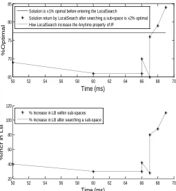
Now we show how this heuristic improves the anytime property of the IP algorithm. For this purpose, we observe the behaviour of the heuristic while it visits each sub-space. To this end, we assume that we have 15 agents and values have been drawn from the NDCS distribution. Furthermore, we want to find a solution which is 85% optimal. It is worthy to note that algorithm will stop only if it is successful in finding the required optimal solution or it has visited all the sub-spaces. The behaviour of the heuristic is shown in fig. 4. In fig. 4, the percent increase in LB (in lower plot) refers to
(𝑳𝑩_𝑹𝒆𝒂𝒍𝑮− 𝑨𝑽𝑮𝑮
𝑨𝑽𝑮𝑮 ) ∗ 100, where 𝐿𝐵_𝑅𝑒𝑎𝑙𝐺 is the solution
computed by the LocalSearch heuristic in a particular sub-space G. The solid line (in the upper plot) shows that the solution is 77% optimal before the IP algorithm calls the LocalSearch heuristic. We record the results after LocalSearch heuristic visits each sub-space (dotted line in the upper plot). Note that the solution becomes 85% optimal (i.e. 𝑥2− 𝑥1=
15 See appendix A.
16 We run our heuristic wth 𝜎 = 0.1. 17
Fig. 3: LocalSearch heuristic for the NDCS distribution. The ‗time (ms) taken by LSA‘ refers to the time LocalSearch heuristic took to compute the solution, and the ‗time (ms) taken by IP‘ refers to the time IP algorithm took to scan the input, search the second level, and run the LocalSearch or GreedySearch heuristic to completion18.
8%, which corresponds to the increase in the solution quality) after visiting a few sub-spaces and then algorithm stops and returns the solution. This behaviour shows that the LocalSearch heuristic improve the anytime property of the IP algorithm.
Note that this heuristic increases the solution quality of the IP algorithm as well. Moreover, the percent increase in the solution quality is at least equal to the percent increase in the LB*19.
B. GreedySearch Heuristic
We plug-in the GreedySearch heuristic in the IP algorithm, run the algorithm for 15 to 27 agents, stop it when the GreedySearch heuristic finishes finding a solution, and record the results. Furthermore, we run our algorithm for 50 times, and reported the average results. The results in the case of NDCS distribution are shown in fig. 5.
Fig. 5 shows that the GreedySearch heuristic is able to find 70 to 75% optimal solutions in less than 400ms. Although the increase in LB* is between 2-4%, but it is a significant improvement, as time taken by it to return a solution is very small. Similar results were observed in the case of normal distribution. Furthermore, for uniform distribution, the results
18
The terms ‗time (ms) taken by LSA‘ and ‗time (ms) taken by IP‘ have the same meaning for all figures.
19
For proof, refer to appendix B.
Fig. 4: How LocalSearch heuristic improves the anytime property of the IP algorithm.
were not statistically significant (The reason is the same, as discussed before).
Note that for 27 agents, this heuristic returns a good-enough solution in 410ms that is 10 times less as compared to the time taken by the IP algorithm (5000ms – 410ms) to scan the input and search the second level. It is worth noting that, for 27 agents and NDCS distribution, finding an optimal solution can take many hours (or days) as shown in fig. 1. Hence, one may prefer a good solution over optimal for setting where one has constraint over time (for instance, in real-time applications).
C. Selection Functions for IP Algorithm
We assume that we want to find a 92% optimal solution20. We recorded the performance of the IP algorithm for 15 to 21 agents against uniform, normal, and NDCS distribution. Furthermore, we run our algorithm 70 times for 15 to 19 agents and 50 times for 20 to 21 agents, and recorded the average results. The results in the case of NDCS distribution are shown in fig. 621.
20 We take this value as an example. Any other value less than 100% can be assumed. Furthermore, nearly similar results were observed for 85% optimal solution.
21 Similar results were observed for normal and uniform distribution.
8 10 12 14 16 18 20 22
75 80 85 90
%
O
p
tim
a
l
8 10 12 14 16 18 20 22
0 200 400
IP
T
im
e
(
m
s
)
8 10 12 14 16 18 20 22
0 100 200 300
L
S
A
T
im
e
(
m
s
)
8 10 12 14 16 18 20 22
0 5 10
Number of Agents
%
In
c
r
in
L
B
*
50 52 54 56 58 60 62 64 66 68 70
65 70 75 80 85
Time (ms)
%
O
p
ti
m
a
l
Solution is x1% opimal before entering the LocalSearch
Solution return by LocalSearch after searching a sub-space is x2% optimal How LocalSearch increase the Anytime property of IP
50 52 54 56 58 60 62 64 66 68 70
20 40 60 80 100 120
Time (ms)
%
In
c
r
in
L
B
[image:6.612.50.289.61.330.2]
Fig. 5: GreedySearch heuristic for the NDCS distribution22.
Fig. 6 shows that, the following sub-spaces are found good in generating the required solution:
Sub-spaces having the highest LB with the smallest size return the solution about 30 to 300% faster than the other ones. The reason is that, they contain overall high values of the coalitions; hence, after searching a few solutions, we may find the desired optimal solution. Furthermore, it is able to return a good solution faster than others due to its smaller size.
Sub-spaces having the highest UB with the smallest size return the solution about 40 to 200% fasters then the rest ones (excluding the highest LB +1/Size) one. The reason is that the highest UB ensures to generate good solution and smallest size ensures that it can be generated much quickly.
Sub-spaces having the smallest size show same behaviour as that of the highest (UB+1/Size) one. The reason is that, they can return solution much quickly due to their smallest size.
Furthermore, some sub-spaces, such as the one having lowest ((UB-LB) + 1/Size) are more than 100% slower in generating the solution. The reason is that, they have large size and low values of the coalitions. From the results, we can conclude that the selection of a particular sub-space has significant effect on the time required to find a good solution.
22 In fig. 5, the ‗time (ms) taken by GSA‘ refers to the time GreedySearch heuristic took to compute the solution
Fig. 6: The time required to generate the 92% optimal solution for different sub-spaces against NDCS distribution.
VI. CONCLUSION AND FUTURE WORK
Coalition formation is an advanced research area within multi-agent systems nowadays. Generally, the goal of the coalition structure generation activity is to maximize the social welfare by finding the optimal coalition structure, but exponential nature of the solution space does not allow making exhaustive search for the optimal solution. Hence, we may prefer a good solution over an optimal one in settings where we have constraints on execution time and memory. From this line of research, we proposed two new heuristics for coalition structure generation.
This paper advances the state of the art in the followings:
First, we proposed a novel heuristic, namely LocalSearch for coalition structure generation and empirically show that it generates good-enough solution in short time. Furthermore, it improves the anytime property, lower bound, and solution quality of the IP algorithm. The increased lower bound can prune a major portion of the exponential search space without going into the space.
Second, we proposed a greedy heuristics, namely GreedySearch for finding a good-enough solution, without going fully to any of the sub-space, in settings where we have a large number of agents (>20).
Third, we implemented different heuristics for selecting a sub-space in the IP algorithm proposed by [12]. We show that, in order to find a good solution (as opposed by optimal), the selection of a particular sub-space in the IP
16 18 20 22 24 26
65 70 75 80
%
O
p
tim
a
l
16 18 20 22 24 26
0 2000 4000
IP
T
im
e
(
m
s
)
16 18 20 22 24 26
0 200 400
G
S
H
T
im
e
(
m
s
)
16 18 20 22 24 26
0 2 4
Number of Agents
%
In
c
r
in
L
B
*
15 16 17 18 19 20 21 22
0 500 1000 1500
Number of Agents
T
im
e
(
m
s
)
Lowest((UB-LB)+1/size) Highest(LB)
Highest((UB-LB)+1/size) Highest (LB)
[image:7.612.315.563.61.324.2]algorithm has significant effect on its performance, in term of the time required to return the solution.
As a future work, we would like to integrate our work with recommender systems [13, 14]. There has been no work in literature that uses coalition formation among agents for solving recommender systems problems. If we divide users (or items) into distinct clusters, then our algorithm can be used in finding the most relevant users (or items). A K nearest neighbour based collaborative filtering algorithm can be used for generating recommendations. Furthermore, proposed algorithm can be helpful in distributed recommender system.
REFERENCES
[1] Caparrós A., Hammoudi A., and Tazdaït T. (2004). On Coalition Formation with Heterogeneous Agents. Working Papers 2004.70, Fondazione Eni Enrico Mattei
[2] Larson H. S., Sandholm T. W. (1999). Anytime coalition structure generation: an average case study, Proceedings of the third annual conference on Autonomous Agents, p.40-47, Seattle, Washington, United States
[3] Sandholm, T. W., Larson, K., Andersson, M., Shehory, O., and Tohme, F. (1999). Coalition structure generation with worst case guarantees. Artificial Intelligence, 111(1–2):209–238.
[4] Rahwan, T. (2007) Algorithms for Coalition Formation in Multi-Agent Systems. PhD thesis, University of Southampton.
[5] Yeh, D. Y. (1986). A dynamic programming approach to the complete set partitioning problem. BIT Numerical Mathematics, 26(4):467–474
[6] Rothkopf, M. H., Pekec, A., and Harstad, R. M. (1995). Computationally manageable combinatorial auctions. Management Science, 44(8):1131–1147.
[7] Rahwan T. and Jennings N. R. (2008b). An improved dynamic programming algorithm for coalition structure generation. In Proc 7th Int Conf on Autonomous Agents and Multi-Agent Systems (AAMAS- 08), Estoril, Portugal , volume 3, pages 1417–1420.
[8] Sen, S. and Dutta, P. (2000). Searching for optimal coalition structures. In Proceedings of the Fourth International Conference on Multiagent Systems, pages 286–292.
[9] O. Shehory and S. Kraus. Methods for task allocation via agent coalition formation. Artificial Intelligence, 101(1–2):165–200, 1998.
[10] V. D. Dang and N. R. Jennings. Generating coalition structures with finite bound from the optimal guarantees. In Proceedings of the Third International Joint Conference on Autonomous Agents and Multiagent Systems (AAMAS), pages 564–571, 2004.
[11] T. Rahwan, S. D. Ramchurn, V. D. Giovannucci, V. D. Dang, and N. R. Jennings. Anytime optimal coalition structure generation. In Proceedings of the Twenty second Conference on Artificial Intelligence (AAAI-07), pages 1184–1190, 2007.
[12] T. Rahwan, S. D. Ramchurn, A. Giovannucci, and N. R. Jennings (2009). An Anytime Algorithm for Optimal Coalition Structure Generation. Journal of Artificial Intelligence Research (JAIR). 34, Pages 521-567.
[13] Mustansar Ali Ghazanfar, and Adam Prugel-Bennett, “A Scalable, Accurate Hybrid Recommender System” , In the 3rd International Conference on Knowledge Discovery and Data Mining (WKDD 2010), 9-10 Jan 2010, Thailand.
APPENDIX A
For benchmarking the coalition structure generation algorithms, the standard instances of the input value distribution have been defined as follows [2]:
Normal Distribution: 𝑣 𝐶 = 𝐶 x 𝑝 where 𝑝 ~ 𝑁 𝜇, 𝜎2 ,
𝜇 = 1 𝑎𝑛𝑑 𝜎 = 0.1
Uniform Distribution: 𝑣 𝐶 = 𝐶 x 𝑝 where 𝑝 ~ 𝑈 𝑎, 𝑏 ,
𝑎 = 0 𝑎𝑛𝑑 𝑏 = 1
Sub-additive: 𝑣 𝐶 ≤ 𝑣 𝐶′ + 𝑣(𝐶′′) where 𝐶 = 𝐶′∪ 𝐶′′ and
𝑣(𝐶) is uniform as above. (In this case the singleton coalitions form the optimal structure)
Super-additive:𝑣 𝐶 ≥ 𝑣 𝐶′ + 𝑣(𝐶′′) where 𝐶′, 𝐶′′𝑎𝑛𝑑 𝑣(𝐶)
are as defined above (In this case the grand coalition is the optimal structure).
The validity of uniform and normal instances has been questioned by [13], where the authors claimed that these instances generate biased results:“we analytically show that
any CSG problem with an input defined according to distributions of coalition values based on the size of the coalitions (such as the Normal and Uniform distributions above) will generate biased results” [13].
In fact this was the main reason why in the case of uniform and normal distribution, our Heuristics (LocalSearch and GreedySearch) did not showed much improvement in the LB* computed by the IP algorithm.
NDCS (Normally Distributed Coalition Structures): This instance of the input distribution has been defined by [12], and is well suited for the coalition structure generation problems. This instance is defined as follows:
𝑣 𝐶 ~𝑁 𝜇, 𝜎2 , where 𝜇 = |𝐶|, 𝜎 = |𝐶|
In this distribution, the value of every possible coalition structure is independently drawn from the same normal distribution
Furthermore, for this distribution, our heuristics showed significant improvement in LB* computed by the IP algorithm.
APPENDIX B
This comes from the fact that LB* = max (𝑨𝑽𝑮𝑮∗, 𝑽(𝑪𝑺′))
where 𝑉 𝐶𝑆′ is the best solution found in
levels 𝔭1, 𝔭2, 𝑎𝑛𝑑 𝔭𝑛. Let 𝐿𝐵_𝑅𝑒𝑎𝑙∗ be the best solution found by the LocalSearch heuristic. We compute the percent increased in the LB* as follow: % 𝑰𝒏𝒄𝒓𝒆𝒂𝒔𝒆 𝒊𝒏 𝒕𝒉𝒆 𝑳𝑩∗= (𝑳𝑩𝑹𝒆𝒂𝒍∗−𝑳𝑩∗
𝑳𝑩∗ ) * 100. We can easily conclude from this
equation that the % increase in the solution quality is at least equal to this % increase in the LB* (in case we have LB*=
![Fig. 1: Example of the integer partition graph for 4 agents [12].](https://thumb-us.123doks.com/thumbv2/123dok_us/1299413.659446/2.612.322.529.52.234/fig-example-integer-partition-graph-agents.webp)
![Fig. 2: The time required to find the optimal solution for IDP and IP under NDCS, Normal, and Uniform Distributions [12]](https://thumb-us.123doks.com/thumbv2/123dok_us/1299413.659446/3.612.57.296.186.379/fig-required-optimal-solution-ndcs-normal-uniform-distributions.webp)