Abstract—The paper presents an original homogenization method to predict the elastic properties of multiphase pre-impregnated composite materials like Sheet- and Bulk Molding Compounds. The upper and lower limits of the homogenized coefficients for a 27% fibres volume fraction SMC are computed. It is presented a comparison between the upper and lower limits of the homogenized elastic coefficients of a SMC material and the experimental data. The estimation model used as a homogenization method of these heterogeneous composite materials, gave emphasis to a good agreement between this theoretical approach and experimental data.
Index Terms—Prepregs, homogenization, elliptic equations, elastic coefficients.
I. INTRODUCTION
The most obvious mechanical model which features a multiphase composite material is a pre-impregnated material, known as prepreg. In the wide range of prepregs the most common used are Sheet- and Bulk Molding Compounds. A Sheet Molding Compound (SMC) is a pre-impregnated material, chemically thickened, manufactured as a continuous mat of chopped glass fibres, resin (known as matrix), filler and additives, from which blanks can be cut and placed into a press for hot press moulding. The result of this combination of chemical compounds is a heterogeneous, anisotropic composite material, reinforced with discontinuous reinforcement [1]–[3].
A typical SMC material is composed of the following chemical compounds: calcium carbonate (36.8% weight fraction); chopped glass fibres rovings (30% weight fraction); unsaturated polyester resin (18.4% weight fraction); low-shrink additive (7.9% weight fraction); styrene (1.5% weight fraction); different additives (1.3% weight fraction);
Manuscript received February 19, 2009. This work was supported in part by the Transilvania University of Brasov, Romania under Grant 135/2007.
H. Teodorescu-Draghicescu is with the Department of Mechanics within Transilvania University of Brasov, Romania (corresponding author to provide phone: +40-268-418992; fax: +40-268-418992; e-mail: draghicescu.teodorescu@)unitbv.ro).
S. Vlase, is with the Department of Mechanics within Transilvania University of Brasov, Romania (e-mail: [email protected]).
A. Chiru is with the Department of Automotives and Engines within Transilvania University of Brasov, Romania (e-mail: [email protected]).
M.L. Scutaru is with the Department of Mechanics within Transilvania University of Brasov, Romania (e-mail: [email protected]).
D.L. Motoc is with the Department of Precision Mechanics and Mechatronics within Transilvania University of Brasov, Romania (e-mail: [email protected]).
pigmented paste (1.3% weight fraction); release agent (1.2% weight fraction); magnesium oxide paste (1.1% weight fraction); organic peroxide (0.4% weight fraction); inhibitors (0.1% weight fraction).
The matrix (resin) system play a significant role within a SMC, acting as compounds binder and being “embedded material” for the reinforcement. To decrease the shrinkage during the cure of a SMC prepreg, filler (calcium carbonate) have to be added in order to improve the flow capabilities and the uniform fibres transport in the mold. For the materials that contain many compounds, an authentic, general method of dimensioning is hard to find. In a succession of hypotheses, some authors tried to describe the elastic properties of SMCs based on ply models and on material compounds [4]–[6].
The glass fibres represent the basic element of SMC prepreg reinforcement. The quantity and roving orientation determine, in a decisive manner, the subsequent profile of the SMC structure’s properties. There are different grades of SMC prepregs: R-SMC (with randomly oriented reinforcement), D-SMC (with unidirectional orientation of the chopped fibres), C-SMC (with unidirectional oriented continuous fibres) and a combination between R-SMC and C-SMC, known as C/R-SMC.
The following information is essential for the development of any model to describe the composite materials behaviour [7]: the thermo-elastic properties of every single compound and the volume fraction concentration of each compound.
Theoretical researches regarding the behaviour of heterogeneous materials lead to the elaboration of some homogenization methods that try to replace a heterogeneous material with a homogeneous one [8]–[10]. The aim is to obtain a computing model which takes into account the microstructure or the local heterogeneity of a material. The homogenization theory is a computing method to study the differential operators’ convergence with periodic coefficients [11]–[13]. This method is indicated in the study of media with periodic structure like SMCs and BMCs. The matrix- and fillers elastic coefficients are very different but periodical in spatial variables. This periodicity or frequency is suitable to apply the homogenization theory to the study of heterogeneous materials.
A SMC material can be regarded as a system of three basic compounds: resin, filler and reinforcement (fibres). We can consider the resin–filler system as a distinct phase compound called substitute matrix, so a SMC can be regarded as a two phase compound material. This substitute matrix presents the virtual volume fractions Vr' for resin and
' f
V for filler. These virtual volume fractions are connected to the real
A Homogenization Method for Pre-Impregnated
Composite Materials
volume fractions Vr and Vf , through the relations: ,
; '
'
f r
f f f r
r r
V V
V V V V
V V
+ = +
= (1)
so that Vr'+Vf' =1.
II. AHOMOGENIZATIONMETHOD
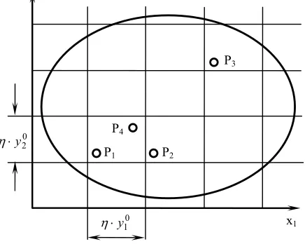
[image:2.612.79.294.234.613.2]We consider Ω a domain from R3 space, in xi coordinates, domain considered a SMC composite material, in which a so called substitute matrix (resin and filler) is represented by the field Y1 and the reinforcement occupies the field Y2 seen as a bundle of glass fibres, (Fig. 1).
Fig. 1. Periodicity definition of SMCs Let us consider the following equation [14]:
ji ij j ij i
a a x
u x a x x
f =
∂ ∂ ⋅ ∂
∂ −
= ( ) ;
)
( (2)
or under the equivalent form: . ;
j ij i i i
x u a p x p f
∂ ∂ ⋅ = ∂
∂ −
= (3)
In the case of SMC materials that present a periodic structure containing inclusions, aij(x) is a function of x. If the period’s dimensions are small in comparison with the dimensions of the whole domain then the solution u of the equation (2) can be considered equal with the solution suitable for a homogenized material, where the coefficients aij are constants.
In the R3 space of yi coordinates, a parallelepiped with yi0 sides (Fig. 1) is considered, as well as parallelepipeds obtained by translation niyi0 (ni integer) in axes directions. The functions:
=
η
η x a x
aij( ) ij , (4) can be defined, where η is a real, positive parameter. Notice that the functions aij(x) are ηY-periodical in variable x (ηY being the parallelepiped with ηyi0 sides). If the function f(x) is in Ω defined, the problem at limit can be considered:
. 0
, ) ( )
( =
∂ ∂ ⋅ ∂
∂ − =
Ω ∂
η
η η
u
x u x a x x f
j ij
i (5)
Similar with equation (3), the vector prη can be defined with the elements:
j ij i
x u x a x p
∂ ∂ ⋅
= η η
η( ) ( ) . (6)
For the function uη(x) an asymptotic development will be looking for, under the form:
, ...; ) , ( ) , ( ) , ( )
( 0 11 2 2
η
η
η
η x
y y x u y x u y x u x
u = + + + = (7)
where ui(x,y) are Y-periodical in y variable. The functions
ui(x,y) are defined on Ω x R3 so that the derivatives behave in the following manner:
. 1
i i
i x y
dx d
∂ ∂ ⋅ + ∂
∂ →
η (8) If the values of
η x x
ui , are compared in two homologous points P1 and P2, homologous through periodicity in neighbour periods, it can be notice that the dependence in
η x
is the same and the dependence in x is almost the same since the distance P1P2 is small (Fig. 2).
Fig. 2. Physical meaning of SMCs inclusions’ periodicity Y1
Y2
Γ
x1 x2
y2
Y 0 1 y 0
2 y
y1 x2
x1
P1 P2
P4
P3
0 2 y ⋅ η
[image:2.612.313.531.534.708.2]Let us consider P3 a point homologous to P1 through periodicity, situated far from P1. The dependence of u
i in y is the same but the dependence in x is very different since P1 and P3 are far away. For instance, in the case of two points P1 and P4 situated in the same period, the dependence in x is almost the same since P1 and P4 are very close, but the dependence in y is very different since P1 and P4 are not homologous through periodicity. The function uη depends on the periodic coefficients aij, on the function f(x) and on the boundary ∂Ω. The development (24) is valid at the inner of the boundary
Ω
∂ , where the periodic phenomena are prevalent but near and on the boundary, the non-periodic phenomena prevail [15].
Using the development (7), the expressions i
x u ∂ ∂ η
and pη
can be computed as following [14]:
(
+ ⋅ +)
= ⋅ ∂ ∂ ⋅ + ∂ ∂ = ∂ ∂ ...1 0 1
u u y x x u i i i η η η ..., 2 1 1 0 + ∂ ∂ + ∂ ∂ ⋅ + ∂ ∂ + ∂ ∂ = i i i i y u x u y u x u η (9) ..., ) , ( ) , ( ) , ( )
(x =p0 x y + ⋅p1 x y + ⋅p2 x y +
pi i η i η i
η (10) where: ... , ) ( ) , ( , ) ( ) , ( 2 1 1 1 0 0 ∂ ∂ + ∂ ∂ ⋅ = ∂ ∂ + ∂ ∂ ⋅ = j j ij i j j ij i y u x u y a y x p y u x u y a y x p (11)
The function f(x) presented in equation (5) can be written in the following manner:
(
...)
.1 )
( ⋅ 0+ ⋅ 1+
∂ ∂ ⋅ − ∂ ∂ −
= i i
i i p p y x x f η
η (12)
The terms η-1 and η0 will be: , 0 0 = ∂ ∂ i i y p (13) . ) ( 1 0 i i i i y p x p x f ∂ ∂ − ∂ ∂ −
= (14) Equation (14) leads to the homogenized- or macroscopic equation. For this, the medium operator is introduced, defined for any function Ψ(y), Y-periodical:
∫
Ψ = Ψ Y dy yY ( ) ,
1
(15) where Y represents the periodicity cell volume. To obtain the homogenized equation, the operator (15) is applied to equation (14): . ) ( 1 0 i i i I y p x P x f ∂ ∂ − ∂ ∂ −
= (16)
According to the operator (15), the second term of the left side of the equation (16) becomes:
∫
∫
∂ = = ∂ ∂ = ∂ ∂ Y i i Y i i ii pnds
Y dy y p Y y p . 0 1
1 1 1
1
(17) Due to Y-periodicity of p1i and the fact that n is the normal vector at the boundary of Y, the relation (17) is equal with zero. So, the equation (16) becomes:
. ) ( 0 i I x P x f ∂ ∂ −
= (18) With help of relation (11), the equation (13) can be written as follows: , 0 ) ( 1 0 = ∂ ∂ + ∂ ∂ ⋅ = ∂ ∂ j j ij i y u x u y a
y (19)
therefore: . ) ( 0 1 j ij j j ij i y a y u y u y a y ∂ ∂ ⋅ ∂ ∂ = ∂ ∂ ⋅ = ∂ ∂
− (20)
The solution u1(y) of equation (20) is Y-periodical and to determine it is necessary to introduce the space
{
u H Y uY periodical}
Y
Uy( )= ∈ ( ), −
1
. The equation (20) is equivalent with the problem to find a solution u ∈Uy
1 that verifies: , ) ( 0 1 vdy y a x u dy y v y u y a Y i ij j i Y j ij
∫
∫
∂ ∂ ∂ ∂ = ∂ ∂ ⋅ ∂ ∂ (21)for ∀v∈Uy. If y k
U ∈
χ is introduced, with χk =0, that satisfy: , ) ( vdy y a dy y v y y a i ik i Y j k ij
∫
∫
∂ ∂ = ∂ ∂ ⋅ ∂ ∂χ (22) for ∀v∈Uy , then from the problem’s linearity (21), its solution can be written under the form:), ( ) ( ) , ( 0
1 y c x
x u y x u k k + ∂ ∂
= χ (23)
where c(x) is a constant as a function of x.
Knowing the expression of u1 as a function of u0, from the expressions (11) with (23), the homogenized coefficients can be computed: . ) ( ) ( ) ( ) ( ) , ( 0 0 0 1 0 0 k j k ij ij j k k j ij j j ij i x u y y a y a y x u x u y a y u x u y a y x p ∂ ∂ ∂ ∂ ⋅ + = = ∂ ∂ ⋅ ∂ ∂ + ∂ ∂ = ∂ ∂ + ∂ ∂ = χ χ (24)
Applying the medium operator (15), the relation (24) can be written: , ) ( 0 0 0 k ik i x u a x p ∂ ∂
. )
(
) ( ) ( 0
j k ij ik j
k jk ij
j k ij ik ik
y a a y
y a
y y a y a a
∂ ∂ + =
∂ ∂ + ⋅
= ∂ ∂ + =
χ χ
δ
χ
(26)
Therefore, the relation (16) becomes an equation in u0 with constant coefficients:
. 0 0
∂ ∂ ∂
∂ − =
k ik
i x
u a x
f (27)
III. APPLICATION FOR ASMC MATERIAL
For a composite material in which the matrix occupies the domain Y1 and presents the coefficient a1ij and the inclusion occupies the domain Y2 with the coefficient aij2 separated by a surface Γ, the equation (4) must be seen as a distribution.
In the case of a SMC composite material which behaves macroscopically as a homogeneous elastic environment, is important the knowledge of the elastic coefficients. Unfortunately, a precise calculus of the homogenized coefficients can be achieved only in two cases: the one-dimensional case and the case in which the matrix- and inclusion coefficients are functions of only one variable. For a SMC material is preferable to estimate these homogenized coefficients between an upper and a lower limit.
[image:4.612.79.281.474.641.2]Since the fibres volume fraction of common SMCs is 27%, to lighten the calculus, an ellipsoidal inclusion of area 0.27 situated in a square of side 1 is considered. The plane problem will be considered and the homogenized coefficients will be 1 in matrix and 10 in the ellipsoidal inclusion. In Fig. 3, the structure’s periodicity cell of a SMC composite material is presented, where the fibres bundle is seen as an ellipsoidal inclusion.
Fig. 3. Periodicity cell of a 27% fibres volume fraction SMC Let us consider the function f(x1, x2) = 10 in inclusion and 1 in matrix. To determine the upper and the lower limit of the homogenized coefficients, first the arithmetic mean as a function of x2-axis followed by the harmonic mean as a function of x1-axis must be computed.
The lower limit is obtained computing first the harmonic mean as a function of x1-axis and then the arithmetic mean as a function of x2-axis. If we denote with φ(x1) the arithmetic mean against x2-axis of the function f(x1, x2), it follows:
(
0,5; 0,45) (
0,45; 0,5)
, ,1 ) , ( ) (
1 5 , 0
5 , 0
2 2 1 1
∪ − − ∈
= =
∫
−
x for
dx x x f x ϕ
(28)
(
0,45; 0,45)
., 2025 , 0 45 , 9 1 ) , ( ) (
1 5 , 0
5 , 0
2 1 2
2 1 1
− ∈
− +
= =
∫
−
x for
x dx
x x f x ϕ
(29)
The upper limit is obtained computing the harmonic mean of the function φ(x1):
.
2025 , 0 45 , 9 1
1 )
( 1 1
45 , 0
5 , 0
45 , 0
45 , 0
5 , 0
45 , 0
1 2 1 1 1
5 , 0
5 , 0
1 1
∫
∫
∫
∫
−
− −
− +
+ − +
+ =
= =
dx x
dx dx
dx x a
ϕ
(30)
To compute the lower limit, we consider ψ(x2) the harmonic mean of the function f(x1, x2) against x1:
(
0,5; 0,19) (
0,19; 0,5)
, ,1
) , (
1 1 )
(
2 5 , 0
5 , 0
1 2 1 2
∪ − −
∈
= =
∫
−x for
dx x x f x
ψ
(31)
(
0,19; 0,19)
., 0361 , 0 42 , 3 1
1
) , (
1 1 )
(
2
2 2 5
, 0
5 , 0
1 2 1 2
− ∈
− −
= =
∫
−x for
x dx
x x f x
ψ
(32)
The lower limit will be given by the arithmetic mean of the function ψ(x2):
∫
∫
∫
∫
− −
−
− −
+ − −
+
+ = =
19 , 0
19 , 0
5 , 0
19 , 0
2 2 2 2 5
, 0
5 , 0
19 , 0
5 , 0
2 2
2
. 0361
, 0 42 , 3 1
) (
dx x dx
dx dx x
a ψ
(33)
Since the ellipsoidal inclusion of the SMC structure may vary angular against the axes’ centre, the upper and lower limits of the homogenized coefficients will vary as a function of the intersection points coordinates of the ellipses, with the axes x1 and x2 of the periodicity cell (Fig. 4).
The micrographs presented in Fig. 5 make obvious this angular variation of the fibres’ bundles, the extreme - 0.5 -
0
.4
5 0.19
- 0.19
0
.4
5
0.5 x1 0.5
heterogeneity and the layered structure of these materials as well as the glass fibres and fillers distribution. The micrographs show that there are areas between 100 – 200 µm in which the glass fibres are missing and areas where the fibres distribution is very high.
Fig. 4. ± 30° angular variation of the ellipsoidal inclusion
Fig. 5. Micrographs of various SMCs [1]
IV. RESULTS
Typical elasticity properties of the SMC isotropic compounds and the composite structural features are presented in table 1.
Table 1. Elasticity properties of SMC isotropic compounds
Property UP
resin
Fibre (E-glass)
Filler (CaCO3) Young modulus E
(GPa) 3.52 73 47.8
Shear modulus G
(GPa) 1.38 27.8 18.1
Volume fraction
(%) 30 27 43
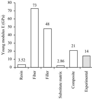
According to the following equations, the longitudinal elasticity moduli ESM (for the substitute matrix) and EC (for the entire composite) can be computed:
. 1 1
2
f f r r SM
V E V E E
⋅ + ⋅
= (34)
). 1
( F
SM F F
C E V E V
E = ⋅ + ⋅ − (35)
A comparison between these moduli and experimental data is presented in Fig. 6.
48
21 14
3.52 2.86
73
0 10 20 30 40 50 60 70 80
R
es
in
F
ib
er
F
il
le
r
S
u
b
st
it
u
te
m
at
ri
x
C
o
m
p
o
si
te
E
x
p
er
im
en
ta
l
Y
o
u
n
g
m
o
d
u
lu
s
E
(
G
P
[image:5.612.86.283.302.728.2]a)
[image:5.612.328.521.350.560.2]Fig. 6. Computed and experimental Young moduli According to equations (30) and (33), the upper and lower limits of the homogenized coefficients for a 27% fibres volume fraction SMC material are computed and shown in table 2.
Table 2. Homogenized coefficients Angular
variation of the ellipsoidal
inclusion
Upper limit a+ Lower limit a_
0° 2.52 0.83
± 15° 2.37 0.851
± 30° 2.17 0.886
[image:5.612.313.539.657.742.2]The results presented in table 2, show that the upper limit of the homogenized coefficients decreases with the increase of angular variation of the ellipsoidal inclusion unlike the lower limit which increases with the increase of this angular variation.
The material’s coefficients estimation depends both on the basic elasticity properties of the isotropic compounds and the volume fraction of each compound. If we write PM, the basic elasticity property of the matrix, PF and Pf the basic elasticity property of the fibres respective of the filler, φM the matrix volume fraction, φF and φf the fibres- respective the filler volume fraction, then the upper limit of the homogenized coefficients can be estimated computing the arithmetic mean of these basic elasticity properties taking into account the volume fractions of the compounds:
. 3
f f F F M
M P P
P
A+= ⋅ϕ + ⋅ϕ + ⋅ϕ (36) The lower limit of the homogenized elastic coefficients can be estimated computing the harmonic mean of the basic elasticity properties of the isotropic compounds:
, 1 1
1
3
f f F F M
M P P
P A
ϕ ϕ
ϕ + ⋅ + ⋅
⋅ =
− (37)
where P and A can be the Young modulus respective the shear modulus. Fig. 7 shows the Young moduli and Fig. 8 presents the shear moduli of the isotropic SMC compounds as well as the upper and lower limits of the homogenized elastic coefficients.
48
14
3.52 2.86
13.77 73
0 10 20 30 40 50 60 70 80
R
es
in
F
ib
er
F
il
le
r
E
(-)
E
(+)
E
x
pe
ri
m
en
ta
l
Y
o
u
n
g
m
o
d
u
lu
s
E
(
G
P
a)
Fig. 7. Young moduli of the homogenized elastic coefficients The presented results suggest that the environmental geometry given through the angular variation of the ellipsoidal domains can leads to different results for same fibres volume fraction. This fact is due to the extreme heterogeneity and anisotropy of these materials. The upper limits of the homogenized elastic coefficients are very close to experimental data, showing that the proposed
homogenization method give better results than the computed composite’s Young modulus determined by help of the rule of mixture.
18
5
1.32 1.12
5.23 28
0 5 10 15 20 25 30
R
e
si
n
F
ib
e
r
F
il
le
r
G
(
-)
G
(
+
)
E
x
p
e
ri
m
e
n
ta
l
S
h
e
a
r
m
o
d
u
lu
s
G
(
G
P
a
)
Fig. 8. Shear moduli of the homogenized elastic coefficients
REFERENCES
[1] H. Teodorescu, S. Vlase, L. Scutaru, F. Teodorescu, “An original approach of tensile behaviour and elastic properties of multiphase pre-impregnated composite materials”. WSEAS Transactions on Appl. and Theoretical Mechanics, Issue 2, vol. 3, Feb. 2008, pp. 53-62. [2] H.G. Kia, Sheet Molding Compounds. Science and Technology.
Hanser, 1993.
[3] G. Milton, The Theory of Composites. Cambridge University Press, 2002.
[4] C. Miehe, J. Schröder, M. Becker, “Computational homogenization analysis in finite elasticity: material and structural instabilities on the micro- and macro-scales of periodic composites and their interaction”.
Comput Methods Appl Mech Eng , 191, 2002, pp. 4971-5005. [5] T.I. Zohdi, P. Wriggers, Introduction to computational
micromechanics. Springer, 2005.
[6] N. Bakhvalov, G. Panasenko, Homogenization. averaging processes in periodic media: mathematical problems in the mechanics of composite materials. Kluwer Academic Publishers, 1989. [7] J.M. Whitney, R.L. McCullough, “Micromechanical Materials
Modelling” in Delaware Composite Design Encyclopedia, vol. 2, ed. by Carlsson, L.A., 1990.
[8] M. Hori, S. Nemat-Naser, “On two micromechanics theories for determining micro-macro relations in heterogeneous solids”.
Mechanics of Materials, 31, 1999, pp. 667-682.
[9] T.J. Barth, T. Chan, R. Haimes, Multiscale and Multiresolution Methods: Theory and Applications. Springer, 2001.
[10] A. Pavliotis, A. Stuart, Multiscale Methods: Averaging and Homogenization. Springer, 2008.
[11] V.V. Jikov, S.M. Kozlov, O.A. Oleynik, Homogenization of Differential Operators and Integral Functions. Springer, 1994. [12] G. Allaire, Shape Optimization by the Homogenization Method.
Springer, 2001.
[13] P.K. Mallik, Fibre Reinforced Composite materials. Manufacturing and Design. Marcel Dekker Inc., 1993.
[14] H.I. Ene, G.I. Pasa, The Homogenization Method. Applications at Composite Materials Theory. Academy Publishing House, Bucharest, 1987 (in Romanian).
[15] S. Vlase, M.L. Scutaru, H. Teodorescu-D., “Some considerations concerning the use of the law of mixture in the identification of the mechanical properties of the composites”, in Proc. of the 6th