Environmental stability: Its effect on stream benthic communities

(1)

ENVIRONMENTAL STABILITY: ITS EFFECT ON

STREAM BENTHIC COMMUNITIES

A thesis

submitted for the degree of

Doctor of Philosophy in Zoology

in the

University of Canterbury

by

Russell G. Death ' /

University of Canterbury

(2)

(3)

ABSTRACT

The effects of environmental stability on benthic community structure were exam-ined at eleven sites (ten streams and a wind-swept lake shore) in the Cass-Craigieburn region, New Zealand. Physicochemical conditions, apart from stabil-ity, were similar at all sites. Epilithic biomass was considerably higher at the more stable sites, but the composition of periphyton communities, and amounts of benthic organic matter present were more strongly influenced by the nature of the riparian vegetation than by stream stability.

Invertebrate species richness and density were markedly higher at the more stable sites, but species evenness peaked at sites of intermediate stability. Sites of high and low stability had species-abundance distributions that were modelled best by the log series distribution, whereas sites of intermediate stability were modelled best by the log normal distribution. Communities were dominated by a common core of taxa at all sites, although their relative abundances changed markedly between sites. Differences appeared to be related to a combination of environmental stability and site location (e.g., in forest or grassland). Persistence of the dominant taxa was high at all sites, but persistence of the entire fauna was higher at the stable sites.

Communities at the more unstable sites appeared to be less complex and were expected to have higher resilience (i.e., ability to recover from disturbances) than those at more stable sites. Analysis of the local stability of community matrices in-dicated that matrices were unstable at all sites, although those at the less stable sites had eigenvalues closer to the stability criterion. These sites also had higher theoretical resilience if eigenvalues beyond the 'criterion for stability were ig-nored. An experimental study of recovery rates in four streams of different stabil-ity did not provide any support for higher resilience at less stable sites, all commu-nities recovered at a similar rate. The composition of invertebrate commucommu-nities at several of the less stable sites could be attributed to simple random colonisation processes; but community structure at the stable sites could not, although the reason for this remains unclear.

(4)

CHAPTER!

(6)

Chapter 1: General Introduction 2

One of the central issues in community ecology throughout this century has been whether or not the collection of species populations in a particular habitat can be considered a structured entity (Roughgarden, 1989). Are they simply the species that happen to arrive at a site, or are they a special subset with properties that allow their coexistence? Answers to these questions were initially split between two schools of thought, one founded by Elton (1933), who believed a community was an organised entity with limited membership, and the alternative view initi-ated by Gleason (1926) that communities resulted from a combination of chance immigrations and the effects of fluctuating and variable environments.

During the 1960s and 70s advances in theoretical ecology, further developed the view that communities were entities oflimited membership structured by com-petition and to a lesser extent predation (Cody & Diamond, 1975). Attempts during the 80s to find empirical support for the concepts and theories proposed in the 1960s and 70s met with limited success, however (Roughgarden, 1989). Be-cause of this, there has been a swing away from the largely deterministic view of community structure to one placing more emphasis on non-equilibrial and sto-chastic processes (Strong et aI., 1984; Diamond & Case, 1986). This swing has not been complete however, and both the empirical (Schoener, 1986a) and theoretical (DeAngelis & Waterhouse, 1987) nature of communities are now seen to be more pluralistic with most lying somewhere on a continuum between the extremes where communities will be structured entirely by deterministic processes, or solely by stochastic processes (Giller & Gee, 1987; Cody, 1989).

Within the context of this debate over the relative importance of stochastic and deterministic forces, the question of what determines species diversity and how this affects community stability (i.e., the ability of the community to persist in the face of disturbances) has been one of the major topics of contention. The stabil-ity / complexstabil-ity dilemma, i.e., whether more or less complex communities have greater stability has also evolved through the latter part of this century (May, 1981; McIntosh, 1987). During the 1950s and 60s it was generally held that more com-plex communities should be more stable (MacArthur, 1955; Elton, 1958), how-ever, the mathematical modelling approaches of the 1970s (e.g., Gardner &

Ashby, 1970; May, 1972) led to the converse view, and now less complex commu-nities are generally considered to be more stable (May, 1981; Pimm, 1982) at least in theory. Debate centring on the stability/complexity relationship has however, also become pluralistic, and it is now acknowledged that both the scale of distur-bances, and the specific nature of the communities will alter the effects of in-creased complexity on stability (e.g., DeAngelis, 1975; Pimm, 1982).

(7)

communities of different types, it incorporates very little information on the struc-tural and functional nature of a community. To this end, the emergence of food web theory (Cohen, 1978) has been seen as a major advance (Roughgarden, 1989). Thus, while it is still possible to compare comrimnities of very different types, much of their structural and functional nature is retained. Food web studies have uncovered a number of general patterns common to a broad spectrum of commu-nities, although the underlying reasons for these patterns are not so clear (Lawton

& Warren, 1988; Lawton, 1989).

Whereas the main stream of ecology has advanced through both the develop-ment of theory and the empirical testing of theories, lotic ecology has until very recently remained an essentially descriptive science, seemingly oblivious to the theoretical basis of ecology as a whole (Barnes & Minshall, 1983; Hildrew &

Townsend, 1987). Nevertheless, although it was slow to develop, a dichotomy between the deterministic and stochastic views of community structure has also arisen in studies of stream invertebrate assemblages. The view that benthic com-munities are most strongly influenced by stochastic forces, such as disturbances has been propounded by some (e.g., Reice, 1985; Lake & Barmuta, 1986; Lake et al., 1988), whereas others (e.g., Hart, 1983; McAuliffe, 1983; Minshall et at., 1985)

have considered that benthic communities lie on a stochastic - deterministic con-tinuum, and that their position on this continuum is related to environmental sta-bility. Proponents of this latter view, also emphasise temporal and spatial scale as important determinants of the relative position of communities along this contin-uum. Even some workers who consider that most stream communities are struc-tured predominantly by stochastic events do admit that it is at least theoretically possible for deterministic communities to develop in more "benign" (sensu Peckar-sky, 1983) environments (e.g., Lake & Barmuta, 1986). The principal bone of contention therefore seems to be whether or not, such benign conditions ever occur in stream environments.

Discussions about lotic community structure have to date been concerned mainly with the importance of competition (Hart, 1983; McAuliffe, 1983) and predation (Peckarsky, 1983, 1984) as structuring forces in benthic communities. Very little consideration has been given to other topics central to discussions in main-stream ecology, such as the stability/complexity dilemma, food web theory, community persistence and resource partitioning. Although some exceptions to this include Bruns & Minshall (1983) (stability/complexity dilemma), Hildrewet at. (1985) (food web theory), Meffe & Minckley (1986) and Townsend et at. (1987)

(community persistence), and Hildrew et at. (1984), Tokeshi (1986), Tokeshi &

(8)

Furthermore, although both the stability/complexity dilemma and food web theory have received considerable theoretical investigation in main-stream ecol-ogy, there have been few empirical studies undertaken to test these theories. Food web investigations in particular appear to be based almost entirely on 113 food webs (of variable quality) collated from the literature (Briand & Cohen, 1987) (although several more recent studies have begun to redress this problem, for example, Pimm & Kitching (1987), Warren (1989) and Winemiller (1990)). One aim of my study was therefore to collect more empirical data relating to food web theory, in particular, what influence environmental stability has on food web struc-ture.

The central objective of my study was therefore to investigate the effect of environmental stability on benthic community structure by comparing communi-ties in streams of differing environmental stability, but similar physicochemical conditions. In particular, I set out to examine whether these communities could be considered unstructured assemblages of chance colonists, or whether differing levels of environmental stability placed or lifted constraints on community struc-ture. That is, do the communities of more unstable streams have any particular characteristics that allow them to persist (if they do) in the face of continual distur-bance.

MEASUREMENT OF ENVIRONMENTAL STABILITY

(9)

structure and changes resources, substrate availability or the physical environ-ment ". Similarly, frequency and intensity of disturbance, are used as defined by White & Pickett (1985) to mean the number of disturbance events per unit time, and the physical force of the event per unit area per unit time, respectively.

In their review of disturbances in lotic systems, Resh et al. (1988) refined this definition to include only those events outside a predictable range of environ-mental variability. This introduces another component of a disturbance, namely its predictability. They considered that predictability must be included in the defi-nition of disturbance because organisms may well be adapted to withstand pre-dictable seasonal fluctuations (although they admit the generality of this conten-tion needs further investigaconten-tion), and therefore do not represent disturbances to the organisms concerned. In my opinion, environmental stability is related to the area, frequency and/or intensity of disturbances, irrespective of how predictable they may be. For example, the most unstable site included in my study had spates (i.e., disturbances) in most months, and on this time scale, the occurrence of these spates can be considered highly predictable. However, they still resulted in the tumbling of stones and the loss Of animals and periphyton. Does this mean a spate in this stream is not a disturbance because it is predictable in time or does it mean that it is a disturbance because these animals have not adapted to it? To the ani-mals displaced or killed, a spate is surely a disturbance, despite its predictability.

It is all very well to define stability and disturbance, but actually measuring them in the field is another matter. The principal aim of my study was to compare the benthic community structure of streams differing in environmental stability. To achieve this it was therefore necessary for me to measure environmental stabil-ity objectively. Having defined a disturbance as anything " ... that disrupts ecosys-tem, community, or population structure and changes resources, substrate availa-bility or the physical environment II it was necessary to know

a priori

whether

changes in any given variable were likely to affect ecosystem, community or popu-lation structure. Unfortunately, although the effects of some environmental vari-ables (e.g., discharge) are relatively clear, this is not always the case.

(10)

variations in water temperature influence aquatic invertebrate life histories, me-tabolism and growth (Sweeney, 1978; Vannote & Sweeney, 1980) and tempera-ture range has been used as a measure of environmental stability in a number of North American studies (e.g., Stanford & Ward, 1983). However, temperature range is also a measure of the constancy of an environmental variable not the frequency or intensity of it's effect.

Substrate movement and temperature variability almost certainly affect ben-thic invertebrates although probably in different ways, however, neither is discre-tely associated with either disturbance frequency or intensity. In order to measure environmental stability at my study sites it was therefore necessary to measure changes in environmental variables rather than the intensity or frequency of dis-crete disturbance events. It was also necessary to measure several such variables as no single variable can provide an all encompassing or consistent measure of stability. I therefore measured six variables to assess environmental stability; substrate movement, the Pfankuch stability index, variation in depth, variation in current speed, temperature range and stream reach tractive force (see Chapter 2 for details).

SPECIFIC AIMS

In addressing my overall objective to investigate the effect of environmental sta-bility on benthic community structure I examined a number of aspects of benthic community structure.

Specific questions addressed in this thesis are:

1) Does environmental stability affect the food base of the communities and if so how?

2) How does environmental stability affect diversity (both species richness and evenness)?

3) Are the species-abundance distributions of these communities related to environmental stability?

4) Do communities in unstable habitats have lower persistence than communi-ties in stable habitats?

5) Do communities in habitats of lower stability have higher theoretical resil-ience; measured using the local stability criteria of their community matrices?

6) If some communities are more resilient than others what community charac-teristics (e.g., complexity) may account for this?

(11)

8) Are changes in resource utilization patterns found with increasing environ-mental stability, and if so could they be the result of competition?

9) Could the observed communities have been created by random colonisation from the available species pool, and could random colonisation also explain re-colonisation patterns following disturbances?

10) Does food web structure in these streams conform to patterns recorded for communities in a wide range of other habitats?

(12)

CHAPTER 2

(13)

Chapter 2: Study Area 9

INTRODUCTION

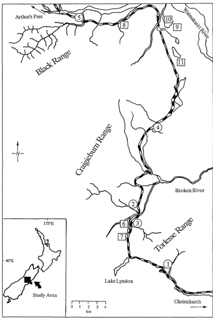
All study sites are small water bodies that eventually flow into the Waimakariri River, in the Cass-Craigieburn region of the Southern Alps, New Zealand (Fig. 2.1).

THE CASS-CRAIGIEBURN REGION

Physical Description

The Waimakariri River catchment was formed when fault movement raised the Southern Alps during the late Tertiary and early Pleistocene, 20 million - 1 million years ago (Hayward, 1974). Late in this period, severe ice action gouged the major faults into river channels giving the catchment its basic shape. This was subse-quently modified by the action of five successive glacial advances, each of which cut the valleys a little deeper. Each time they withdrew, they exposed steep greywacke (hard grey sandstone) and argillite (dark grey mudstone) mountain slopes to the wind, rain and frost. The resulting shattered rock fragments then either moved downslope to accumulate as screes, or were regrouped by the rivers into alluvial fans and terraces.

Soils were formed as the mountain slopes eroded, allowing the establishment of plants, initially on the more stable slopes, but later in the steeper areas. By the time Polynesians occupied Canterbury, forest (beech in the upper reaches merging with podocarp and broadleaf on the eastern foothills) covered most of the land below 1,200-1,400 m, with scrub and grassland above (Burrows, 1960; Moar & Lintott, 1977). Following human occupation, this vegetation suffered at the hands of both Polynesians and Europeans through fire, grazing and the introduction of exotic plants (Relph, 1958; Molloy, 1969). These events in combination with earthquakes and the repetitive freeze-thaw cycle (daily temperature extremes from below freezing to above 30°C during summer) led to a continuing period of erosion and scree formation with beech forests being replaced, except in small patches, by secondary scrub and tussock (Relph, 1957; Burrows, 1960). More detailed infor-mation on the geology, geography and flora of the region can be found in Burrows (1977).

Climate

(14)

t

-N-I

Study Area

I I I I I o 1 2 3 4

km

Broken River

[image:14.530.54.472.64.688.2]

Christchurch

(15)

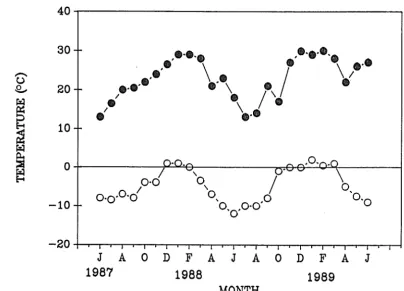
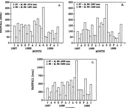
distributed relatively evenly throughout the year (Greenland, 1977). Air tempera-ture at the Craigieburn Forest Meteorological Station, for 1964-1980, ranged from -9.6°C to 32.9°C, with a mean of 8°C for the same period (New Zealand Meteoro-logical Service, 1983). The monthly range at the Cass Field Station over the study period (June 1987 - June 1989) is given in Fig. 2.2. Snow falls on a few occasions in most winters, but seldom persists for more than a few days at any of the study sites. The catchment exhibits a wide range in annual rainfall from east to west, with annual precipitation at Arthur's Pass, 10 km west of Bruce Stream (the most westerly site), five times greater than the annual mean (100 cm) at Kowai River (the most easterly site) (Greenland, 1977). Consequently, there can be marked differences in micro-climate between individual valley basins. Rainfall records for the study period, from climate stations closest to each of the three main valleys are given in Fig. 2.3.

THE STUDY SITES

Introduction

Study sites were chosen to represent a range of streams (small, large, forested, and open) that would differ primarily with respect to the variability of their physical

---

C,) .e,

rz:I

~

rz:I

fil

~

40

30

--20

10

0

10

-•.•.•

,

•.•.•.•

.

.•

.'

\

.

\

/

•.•

'

.

/

•.•.•

•.

\ .

.

/

.

/

\

.

\

.

~

..

D·O.", _=-,,",.0'(,).0

.I

~, ~.Y"'" '-" \

0·0 0 /

O / '0 0'0

0'0' '0 0

'0 0·0' '0 '0'

-20+-rj-r.-~~-r~'-~~'-TJ~-~,-,~,-~~,-~~

J

A

1987

o

D F A

1988

J A

MONTH

o

D F A

J [image:15.527.55.459.431.722.2]

1989

(16)

350~---,

300

I. 87 - lL 88: 1514 mIn

I. 88 - lL 89: 1481 mIn A.

350~---,

I. 87 - K. 88: 1297 mIn _B.

300 J. 88 - K. 89: 1448 mIn

-_~ 250 200

250

200

I

150

100

150

100

J A 0 D F A J A 0 D F A J J A 0 D F A J A 0 D F A J

1987 1988 1989 1987 1988 1989

MONTH MONTH

1250~---,

1000

750

500

J. 87 - lL 88: 4226 mIn 1.88 -lL 89: 54G2 mIn

J A 0 D F A J A 0 D F A J 1987 1988 1989

MONTH

[image:16.528.45.470.61.426.2]

c.

Figure 2.3. Monthly rainfall records between June 1987 and June 1989. A. Craigieburn Forest Park (altitude = 914 m a.s.l) (data courtesy T. McSeveny, Forest Research Institute), B. Chilton Valley, Cass (altitude = 780 m a.s.l.) (data courtesy A. Sturman, University of Canterbury), C. Arthur's Pass (altitude = 738 m a.s.l.) (data courtesy M. Davies, Department of Conservation) (* - data missing).

characteristics. This meant that initially, streams were categorised as "stable" or "unstable" based on the nature of their sources. Those that arose from either a spring or lake outlet were reasoned to be relatively stable, whereas streams without any such point source were reasoned to be comparatively unstable. The stony, wave-washed, southwestern end of Lake Grasmere was also included in the study because it appeared to be a stable environment that superficially resembled a stream, and has a fauna similar to that of streams in the region (Stout, 1977). The altitude and location of each of the study sites is given in Table 2.1.

Unstable Sites

Kowai River (Plate 2.1)

(17)

[image:17.528.107.385.82.359.2]

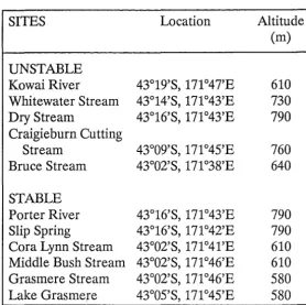
Table 2.1. Map location and altitude of the study sites.

SITES Location Altitude

(m)

UNSTABLE

Kowai River 43°19'S,171°47'E 610

Whitewater Stream 43°14'S, 171°43'E 730

Dry Stream 43°16'S, 171°43'E 790

Craigie burn Cutting

Stream 43°09'S, 171°45'E 760

Bruce Stream 43°02'S, 171°38'E 640

STABLE

Porter River 43°16'S, 171°43'E 790

Slip Spring 43°16'S, 171°42'E 790

Cora Lynn Stream 43°02'S, 171°41'E 610 Middle Bush Stream 43°02'S, 171°46'E 610 Grasmere Stream 43°02'S, 171°46'E 580

Lake Grasmere 43°05'S, 171°45'E 580

the channel at this study site changed repeatedly during the course of the study, moving distances of up to 5 m in the one month interval between visits to the site.

Whitewater Stream (Plate 2.2)

A third order braided stream occupying a 40 m wide flood plain, it drains a catchment of predominantly tussock scrub which is grazed by sheep and cattle for much of the year. The stream channel moved once during the course of the study, the original two channels merging into one and shifting 20 m as a result of a major spate in September 1988.

Dry Stream (Plate 2.3)

A small second order stream occupying a 50 m wide flood plain. Dry stream also drains a catchment of predominantly subalpine tussock scrub, bare scree, and remnant patches of mountain beech. The site dried up periodically during both summers of the study (December-April). The channel changed position once during the study, moving to a new position 5 m from the original after a spate in July 1988.

Craigiebum Cutting Stream (Plate 2.4)

(18)

Plate 2.1. Kowai River

Plate 2.2. Whitewater Stream

(19)

the study site. The stream here has a fairly complete canopy, is well shaded, and

receives comparatively high allochthonous inputs from the overhanging vegetation

(Rounick & Winterbourn, 1983a). Debris dams and pools were present but sparse, and changed position considerably during the course of the study.

Bruce Stream (Plate 2.5)

A third order braided stream occupying a 100 m wide flood plain, it drains a

catchment of predominantly mountain beech and several stands of Monterey pine (Pinus radiata). Channel position changed radically and regularly during the course of the study, moving distances of up to 20 m laterally on at least one occasion.

Plate 2.4. Craigieburn Cutting Stream

(20)

Stable Sites

Slip Spring (Plate 2.6)

This site is the rheocrene/holocrene spring source of the Porter River, arising at the base of a large scree and flowing through tussock grassland before flowing into Porter River. The springbrook is colonised by extensive growths of Myriophyllum sp. and Callitriche stagnalis, both of which are periodically grazed by cattle. Be-cause of this, sampling sites did not include weed beds.

Porter River (Plate 2.7)

An un-named, second order tributary of the Porter River proper, fed by two rheo-crene/holocrene springs, one of which is Slip Spring. It runs through tussock grassland for its entire (1.6 km) length.

Cora Lynn Stream (Plate 2.8)

A first order, spring-fed stream draining a catchment of predominantly matagouri (Discaria toumatou) and tussock scrub. The stream runs through tussock grass-land at the study site but passes through thick matagouri scrub just prior to this.

Middle Bush Stream (Plate 2.9)

The other forested site in the study, this stream is located in the Cass Basin. It is a first order stream that drains a 28 ha catchment of subalpine scrub, tussock and bare scree. The stream has a rheocrene spring source and enters a 3-4 ha stand of mountain beech within which the study site was located. Below the forest it usu-ally flows underground before discharging into Grasmere Stream. Middle Bush Stream is well shaded and its bed consists of alternating pools (caused by log debris dams) and riffles. Forest litter enters the stream year round with a maxi-mum in the summer half of the year (Winterbourn, 1976). Sampling was confined to riffles.

Grasmere Stream (Plate 2.10)

The outlet of Lakes Sarah and Grasmere, this stream flows through tussock grass-land for much of its length but passes through a bed ofPhormium tenax and Typha orientalis just before the study site.

Lake Grasmere (Plate 2.11)

(21)

Plate 2.6. Slip Spring

Plate 2.7. Porter River

(22)

Plate 2.9. Middle Bush Stream

Plate 2.10. Grasmere Stream

(23)

advance, about 16,000-13,000 years before present (Gage, 1959, 1977). A 63 ha lake, its 1,850 ha catchment is primarily tussock grassland, 50% of which is used for agriculture (Gibson, 1978). At the stony, southwestern end of Grasmere, the lake is exposed to extensive wind-induced wave action. The study site was a 20 m stretch of this exposed shore which also receives water from numerous small springs.

PHYSICOCHEMICAL CHARACTERISTICS

Introduction

A number of physical and chemical parameters were measured at each site during the course of the study in order to investigate differences between the "stable" and "unstable" site groups. This was done to establish whether the two groups of streams differed with respect to various physicochemical characteristics and/ or the stability (i.e., variability) of these characteristics.

Materials and Methods

Physical characteristics

Spot records of depth and current speed were obtained monthly between October 1987 and May 1989. Measurements were made near the centre of the stream at a marked point, so that temporal variability could also be assessed. This was achieved by calculating the absolute difference between the measurement in one month and that in the preceding month for all recorded months. Current speed was measured with a Pygmy Gurley current meter, or by recording the time taken for a cork to travel 2 m when the meter failed to function, or flow was too low for it to operate.

A comparative estimate of discharge at each of the study sites was made in November 1989. This was calculated by measuring current speed with a Pygmy Gurley current meter, midway between the surface and the stream bed, and multi-plying this by the stream cross-sectional area. Slope was measured by recording the fall in height along a 20 m section of stream, with an Abney level.

Maximum-minimum and/or spot water temperatures were recorded monthly between October 1987 and May 1989. However, the number of recordings made varied considerably between sites. This was because maximum-minimum ther-mometers were frequently buried or washed away at the more unstable sites, and in May 1988 I gave up using them at Kowai River and Bruce Stream.

(24)

by measuring the three main axes of 100 randomly selected stones (Le. particles

greater than 0.5 cm) from each stream (Newbury, 1984). Half the stones were

collected from randomly assigned, grided 0.5 m2 _{quadrats (the stones were}

col-lected from the intersection points of the 10 cm2 _{grids) and the other half with a}

cross-sectional transect. Mean particle size, geometric mean particle size and

geometric variance were calculated for bed materials at each site (Shirazi & Seim, 1979).

Chemical characteristics

Conductivity and pH of water samples were recorded approximately monthly

between January 1988 and May 1989. Samples were collected in opaque,

polyeth-ylene bottles and stored in the dark at 5°C until analysis could be undertaken (this

was always within 24 hours). Conductivity was measured with a Radiometer CDM

2e conductivity meter and recordings were converted to equivalent values at 25°C

using the appropriate conversion factor (Golterman, 1970). Water pH was

measured with a Metrohm 632 pH meter.

Alkalinity of water samples was measured between February and November

1989 (five samples covering each ofthe seasons) as described by Mackereth (1963).

Concentrations of nitrate-nitrogen (N0₃-N) in water samples collected in March 1988 and November 1989 were measured with the cadmium reduction

alpha-napthylamine-sulfanilic acid technique using the Hach Chemical Company

reagent NitraVer V (accurate to 0.5 mg 1-1). Absorbances were measured on a Kontron Spectrophotometer at 525 nm and converted to nitrate-nitrogen

concen-trations using a standard curve.

Pfankuch stability index

The stability of each stream was evaluated using the stream reach inventory and

channel stability evaluation technique of Pfankuch (1975). This is based on

hydrologic aspects of the channel and streambank, and is essentially a hydrological

engineers tool used for assessing the stability of 2nd to 4th order, forested mountain

streams in the U.S.A. Eifert & Wesche (1982) found it was a useful technique for

evaluating the suitability of habitat for salmonid populations in the U.S.A. and the

procedure has been used to assess stream bed stability in a number of studies in

New Zealand (e.g., Rounick & Winterbourn, 1982; Winterbourn & Collier, 1987; Graesser, 1988), and overseas (Trotter, 1990).

The technique involves rating fifteen variables in three regions of the stream

channel- the upper banks, lower banks and stream bottom according to

(25)

1982). These are summed to give an overall index that evaluates " ... the resistive capacity of mountain stream channels to the detachment of bed and bank materi-als and to provide information about the capacity of streams to adjust and recover from potential changes in flow and/or increases in sediment production... II

(Pfankuch, 1975). The index ranges from a low of 52 (most stable) to a high of 152 (least stable). Because of the subj ective nature of the assessments that make up the index, four people (including myself), all of whom had used the index before, rated each of the study sites. The results were then averaged.

Substrate movement

Although the Pfankuch stability index has been used previously in studies of debris retention (Trotter, 1990), invertebrate community structure (e.g., Rounick &

Winterbourn, 1982; Winterbourn & Collier, 1987; Graesser, 1988), and to charac-terise fish habitat (Eifert & Wesche, 1982), it measures environmental stability on a relatively coarse scale (i.e., the stream reach) which is unlikely to be directly relevant to stream invertebrates. Although this problem may be partly circum-vented by only using the third of the index related to the actual stream bed (i.e., the bottom component), this still relies on a "one-off', somewhat subjective assessment of stream bed stability. A direct measurement of actual substrate movement, the scale at which forces affecting invertebrate community dynamics are most likely to be acting, should therefore be more appropriate.

I obtained such a measure by recording the movement of marked stones within the stream bed. Five fluorescentlypainted stones in each of three size classes (small

<

55 mm; medium 55-90 mm; large, 90-180 mm longest diameter) were placed at a marked point in the stream. Every month between December 1987 and May 1989 the distance travelled by each of the stones was recorded. To convert these data to a single measure of stream substrate movement, the distance travelled by each stone was multiplied by the mean weight of stones in that size class and summed for all stones at that site. On any occasion that a stone was not recovered, an arbitrary distance of 50 m was assigned to the distance travelled, as this was the maximum distance at which a stone was recovered. The value obtained was then converted to a percentage scale, by dividing the actual measure by the maximum possible score (Le., 405.5 kg m, achieved if all stones disappeared), so that 0

=

no stones moved and 100 = all stones disappeared. Each month, all stones were returned to the starting point or replaced if they had disappeared.

Measurement of tractive force

(26)

and/ or move to). However, it is possible to calculate the theoretical proportion of particles that should be moving in uniform flow conditions within the entire stream reach by calculating the streams tractive force.

A column of moving water exerts a force on the stream bed parallel to the slope of the channel, such that if it exceeds a critical value it will set substrate material and organisms in motion. The tractive force of a stream reach T, can be related to the specific weight of water (1000 kg m-3), depth of flow D (m), and the slope of the stream channel S, so that T

=

1000.D.S (kg m-2) (Newbury, 1984).

The critical tractive force (that at the point of incipient motion) for rounded, noncohesive particles > 0.5 cm diameter is approximately equal to the diameter of the particle (cm) (Lane, 1955). Given the particle size distribution of a stream reach it is therefore possible to calculate what proportion of the particles should be moving in uniform flow conditions at a given depth. The tractive force for each of the study reaches was measured, and using the particle size distribution data collected as described above, the percentage of substrate predicted to be moving at any point in time was calculated.

Analysis

To assess whether the two groups of streams were different with respect to individual physicochemical parameters and/or stability measures, all measured variables were analysed with a three level mixed model (factor A & B fixed, factor C random) analysis of variance (ANOV A) using SAS (1985). For the analysis of physical parameters the streams were treated as nested effects, however, for all subsequent analyses the streams were grouped together based on their size, geographic location and whether they were open or forested. To investigate differences based on a number of these variables together, multiple analysis of variance (MANOV A), cluster analysis (using Euclidean distance measures and a group average clustering algorithm), and principal components analysis (PCA) were employed. MANOVA was carried out with SAS (1985), whereas PCA and cluster analysis were carried out with the PC-ORD multivariate statistics package (McCune, 1987).

Results

Physical characteristics

(27)

[image:27.527.61.468.111.532.2]

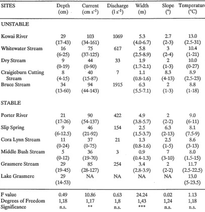
Table 2.2. Physical characteristics of study sites (mean values with the range below in parentheses). F values testing the null hypothesis that stable and unstable sites were similar with respect to these variables are also given. NA = not applicable.

SITES Depth Current Discharge Width Slope Temperature

(cm) , (cms-l) (I s-l) (m)

CO)

COC)

UNSTABLE

Kawai River 29 103 1069 5.3 2.7 13.0

(17-43) (34-161) (4.0-6.7) (2-3) (2.5-31)

Whitewater Stream 16 75 617 5.8 3 10.4

(6-25) (37-125) (2.5-8.9) (2-4) (1-21)

Dry Stream 9 44 33 1.9 2 10.0

(0-19) (0-90) (1.7-2.1) (1-3) (0-27)

Craigieburn Cutting 8 40 7 1.1 8.3 8.9

Stream (4-15) (15-87) (0.8-1.6) (4-13) (2.5-23)

Bruce Stream 34 94 1915 6.3 2 8.8

(13-60) (44-143) (5.5-7.1) (1-3) (1-18)

STABLE

Porter River 21 90 422 4.9 2 9.0

(17"26) (54-137) (3.8-5.7) (2-2) (6-11)

Slip Spring 9 46 154 2.5 6.3 8.1

(6-12.5) (21-92) (1.5-3.7) (2-13) (7.5-9)

Cora Lynn Stream 11 37 21 1.3 2.5 8.6

(0-24) (0-75) (0.8-1.6) (1-5) (3-13)

Middle Bush Stream 5 36 3 0.9 7 8.0

(0-12) (19-70) (0.4-1.3) (3-10) (1.5-15)

Grasmere Stream 29 85 254 3.4 2 11.7

(19-45) (28-127) (2.8-3.9) (2-2) (2.5-22.5)

Lake Grasmere 29 NA NA NA NA 13.0

(14-53) (5-23.5)

F value 0.49 10.86 0.63 24.24 0.02 1.13

Degrees of Freedom 1,18 1,17 1,8 1,43 1,24 1,18

Significance n.s. _** n.s. _*** n.s. n.s.

(28)

Chapter

2:

Study Area

24

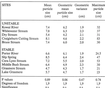
Substrate characteristics of the study sites are given in Table

2.3.

All of the sites were remarkably similar in this respect, with mean particle size between

4.7

and

8.5

cm. None of the substrate parameters were significantly different between the two groups of streams.

Overall differences between stable and unstable stream groups, based on all the physical variables (standardised to a mean of 0 and a standard deviation of 1) were non significant (Wilks' Lambda =

0.01,

F =

23.44,

df =

8,1,

P >

0.05).

Chemical characteristics

[image:28.527.54.468.412.759.2]

A summary of chemical characteristics of the study sites is given in Table

2.4.

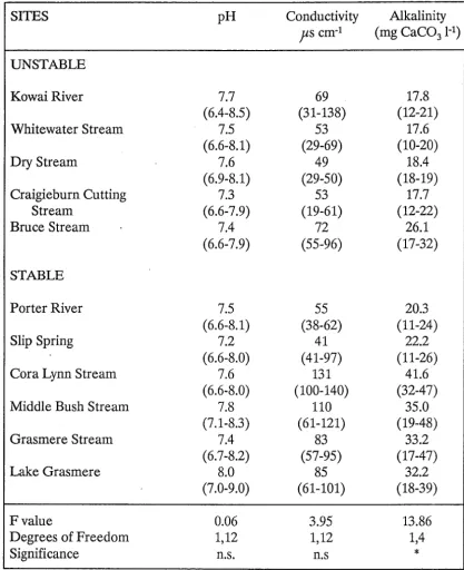
All sites had circumneutral pH (means between

7.2

and

8.0)

and moderate conductivi-ties, although some high values were recorded at a few sites during very low summer flows. Conductivity and pH were not significantly different between the stable and unstable site groups. Alkalinity however, was significantly different between the two groups, although only at the 5% level (means of

31

and

20

mg CaC0₃I-1 for stable and unstable site groups, respectively). Nitrate-nitrogen (N0₃-N) concen-trations at all the sites were below detectable levels

«

0.5

mg 1-1). Reactive phosphorus (P0₄-P) concentrations at a number of these sites, were also found to Table 2.3. Substrate characteristics of the study sites. F values testing the null hypothesis that stable and unstable sites are similar with respect to these variables are also given.

SITES Mean Geometric Geometric Maximum

particle mean vanance particle

size particle size size

(cm) (cm) (cm) (cm)

UNSTABLE

Kowai River

7.4

6.2

1.9

32

Whitewater Stream

7.8

6.3

2.3

37

Dry Stream

5.4

4.2

2.1

31

Craigieburn Cutting Stream

8.1

4.6

2.2

83

Bruce Stream

7.4

6.0

2.0

30

STABLE

Porter River

6.6

6.1

1.9

24.5

Slip Spring

8.5

6.4

2.4

47

Cora Lynn Stream

7.2

5.5

2.0

53

Middle Bush Stream

6.4

4.9

2.3

30

Grasmere Stream

4.7

4.3

1.7

21

Lake Grasmere

5.7

4.7

1.7

23

Fvalues

0.89

0.06

0.47

0.74

Degrees of freedom

1,9

(29)

Table 2.4. Chemical characteristics of the study sites (mean values with the range below in parentheses; conductivity values are medians). F values testing the null hypothesis that stable and unstable sites were similar with respect to these variables are also given.

SITES pH Conductivity Alkalinity

Jls

cm-1 (mg CaC0₃1-1)

UNSTABLE

KowaiRiver 7.7 69 17.8

(6.4-8.5) (31-138) (12-21)

Whitewater Stream 7.5 53 17.6

(6.6-8.1) (29-69) (10-20)

Dry Stream 7.6 49 18.4

(6.9-8.1) (29-50) (18-19)

Craigieburn Cutting 7.3 53 17.7

Stream (6.6-7.9) (19-61) (12-22)

Bruce Stream 7.4 72 26.1

(6.6-7.9) (55-96) (17-32)

STABLE

Porter River 7.5 55 20.3

(6.6-8.1) (38-62) (11-24)

Slip Spring 7.2 41 22.2

(6.6-8.0) (41-97) (11-26)

Cora Lynn Stream 7.6 131 41.6

(6.6-8.0) (100-140) (32-47)

Middle Bush Stream 7.8 110 35.0

(7.1-8.3) (61-121) (19-48)

Grasmere Stream 7.4 83 33.2

(6.7-8.2) (57-95) (17-47)

Lake Grasmere 8.0 85 32.2

(7.0-9.0) (61-101) (18-39)

Fvalue 0.06 3.95 13.86

Degrees of Freedom 1,12 1,12 1,4

Significance n.s. n.s

*

be below detectable levels

«

0.04 mg P) in a previous study (Winterbourn & Fegley, 1989).

No overall differences were found between the two groups of streams based on these chemical parameters (standardised to a mean of 0 and a standard deviation of 1) (Wilks' Lambda

=

0.45, F

=

2.80, df

=

3,7, P > 0.05).

Overall physicochemical differences

[image:29.527.51.468.113.625.2]

(30)

transformation), including stream order and the nature of the stream canopy (Fig. 2.4), split the sites into two principal groups, reflecting a division between small and large streams, rather than stable and unstable ones. Streams in the "large" group were all open streams between 3 and 6 m wide, 16-34 cm deep, and with mean current velocities between 75 and 102 cm S-1. In contrast, the "small" group comprised streams between 0.9 and 2.5 m wide, 5-11 cm deep, and with mean current speeds of 36-46 cm S-1. The latter group also included the lake, probably because many of the variables, such as current speed, could not be measured there. Differences between sites with regard to their overall physicochemical character-istics therefore appeared to be related more to the size and location of the site than its perceived stability.

Variability in physical characteristics

Average differences in spot measurements of depth and current speed at each site in consecutive months are given in Table 2.5. Mean differences in depth ranged from 3 cm at Craigieburn Cutting to 19 cm at Bruce Stream (unstable sites), and from 2 cm at Slip Spring to 7 cm at Lake Grasmere (stable sites). Mean differences in current speed ranged from 18 cm S-l at Craigieburn Cutting to 46 cm S-l at Bruce

Stream (unstable sites), and from 11 cms-1 _{at Middle Bush Stream to 34 cm}_S-l_at

Grasmere Stream (stable sites). Both parameters were significantly greater for the unstable site group.

0.028

I

KowaiRiver

Porter River

Whitewater Stream

Grasmere Stream

Bruce Stream

Dry Stream

Slip Spring

Craigieburn Cutting

Cora Lynn Stream

Middle Bush

Lake Grasmere

1

J

~

0.337

I

DISTANCE 0.647

I 0.956 I

(31)

Table 2.5. Mean monthly variation in depth, current velocity and temperature for the study sites (ranges for these measures are given below in parentheses). F values testing the null hypothesis that stable and unstable sites have similar variation in these factors are also given. NA = not applicable.

SITES Monthly Monthly Monthly

Variation Variation Temperature

of Depth of Current Range

(cm) (cm S-l) eC)

UNSTABLE

Kowai River 7 44 9.8

(0.5-21) (10-99) (3.5-24)

Whitewater Stream 4 27 9.8

(0-14) (0-69) (5.5-14)

Dry Stream 6 35 9.8

(0-15) (0-81) (6-18)

Craigieburn Cutting 3 18 5.8

Stream (0-8) (0-67) (0.5-13.5)

Bruce Stream 19 46 904

(1-42) (1-100) (7-12)

STABLE

Porter River 3 29 2.2

(0-7) (3-83) (1-4)

Slip Spring 2 18 0.5

(0-6) (1-43) (0-3)

Cora Lynn Stream 4 13 2.5

(0-12) (0-41) (1-5)

Middle Bush Stream 3 11 5.7

(0-10) (0-49) ( 4-8.5)

(}rasmereStream 4 34 6.3

(0-15) (1-78) (3.5-12)

Lake (}rasmere 7 NA 8.4

(0-20) (1-13)

Fvalue 29.70 12.81 70040

Degrees of freedom 1,17 1,16 1,17

Significance *** *** ***

Mean monthly temperature range is also given in Table 2.5. It was between 5.8°C and 9.8°C at the unstable sites and O.5°C and 804°C at the stable sites. Temperature range was also significantly greater at the unstable sites.

Pfankuch stability index:

(32)

compo-Chapter 2: Study Area 28

nents are given in Table 2.6. Total index scores ranged from a high of 122 at Kowai River to a low of 64 at Slip Spring. All four measurements were significantly higher for the streams in the unstable site group than those in the stable site group.

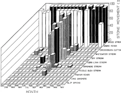
Substrate movement

Distances moved by stones at each of the sites are plotted in Fig 2.5. There appeared to be a good relationship between these measures and my obseryations of high discharge events. Two spates in May and September 1988 (corresponding to the Greymouth flood events), caused major physical changes at several of the sites and these stand out clearly in the monthly plots. Overall, the stable sites had little or no substrate movement. However, the two most unstable sites (Kowai River and Bruce Stream) had all the stones disappearinmostmonths, and the other unstable sites had intermediate levels of substrate movement, which occurred principally in the winter months (May - September).

Mean movement values are summarized in Table 2.7 and ranged from 0 at Slip Spring (where there was no recorded stone movement) to 97 at Bruce Stream (where all stones disappeared in most months). Again the unstable sites had significantly higher measures than the stable sites.

Table 2.6. pfankuch stability index scores with F values testing the null hypothesis that these scores were similar for stable and unstable sites.

SITES Total Upper Bank Lower Bank Bottom

component component component

UNSTABLE

Kowai River 122.25 36.5 36 49.75

Whitewater Stream 110.25 34 37.75 38.5

Dry Stream 106.25 29.5 33.75 42

Craigieburn Cutting 108.25 30 34 44.25

Stream

Bruce Stream 115.75 26.75 39 50

STABLE

Porter River 70.25 17.75 21.5 31

Slip Spring 64 16 17 31

Cora Lynn Stream 68.25 13.75 24 30.5

Middle Bush Stream 111.75 36 34 41.75

Grasmere Stream 74.25 12.75 25.75 35.75

Lake Grasmere 70.25 14 26 30.25

Fvalue 104.39 114.76 53.24 26.11

Degrees of freedom 1,33 1,33 1,33 1,33

(33)

MONTH

I-Z W

L

W

>

o

L

W

Z

o

I-m

[image:33.532.53.476.82.407.2]

STREAM

Figure 2.5. Stone movement measurements (expressed as a percentage of the maximum recordable movement) for each of the study sites between December 1987 and May 1989.

Tractive force measurements

Tractive force measurements obtained for each site, and the percentage of the substrate predicted to move at such a tractive force, are given in Table 2.7. Tractive force ranged from 2.3 to 9.1 kg m-2, and between 13 and 76% of the substrate was predicted to be moving in linear flow and mean depth. Neither critical tractive force nor the percentage of substrate predicted to be moving was significantly different between the two groups of streams.

Overall stability

(34)

Table 2.7. Mean stone movement measures, tractive force and the percentage of the substrate predicted to move given the tractive force. F values testing whether these variables were significantly different between stable and unstable groups are also given. NA = not applicable.

SITES Stone movement Tractive force Percentage of

measure substrate moved by

(%) kgm-2 _{tractive force}_(%)

UNSTABLE

KowaiRiver 63.79 8.09 72

Whitewater Stream 17.21 4.13 28

Dry Stream 11.98 4.10 50

Craigieburn Cutting 18.59 6.07 66

Stream

Bruce Stream 96.86 9.06 70

STABLE

Porter River 0.67 7.24 68

Slip Spring 0.00 8.65 63

Cora Lynn Stream 6.26 7.45 76

Middle Bush Stream 1.37 6.65 68

Grasmere Stream 2.97 2.30 13

Lake Grasmere 0.02 NA NA

Fvalue 62.80 0.01 0.00

Degrees of freedom 1,17 1,8 1,8

Significance

***

n.s. n.s.

Table 2.8. Correlation (r) of mean stability measures with each other. * indicates significance at the 5% level.

STABILITY Depth Current Temperature Stone Total Bottom Predicted MEASURE variability variability range movement Pfankuch component substrate index Pfankuch movement

Depth variability 1.00

Current variability 0.75* 1.00

Temperature range 0.56 0.66* 1.00

Stone movement 0.94' 0.74* 0.60 1.00

Total Pfankuch index 0.49 0.41 0.85' 0.62 1.00

Bottom component of 0.68* 0.58 0.80' 0.80' 0.92'

Pfankuch index

Predicted substrate 0.18 -0.18 -0.30 0.28 0.09 0.16 1.00

movement of tractive force

substrate movement data nor my general observations support the prediction that a high percentage of the substrate materials> 0.5 em diameter was in fact moving at many of my study sites. It therefore appears, that in these streams at least, critical tractive force is not a very useful predictor of substrate stability.

(35)

temperature range, and therefore they too did not appear to reflect the overall physicochemical stability of a site. Many of the criteria used to obtain the index relate to the probability of hydrologic stability and do not necessarily measure actual variations in the environment. For example, the water level in Porter River is always just a few centimetres below bankfull, a highly unstable criterion according to the Pfankuch procedure. However, the stream is spring-fed and the flow never increases much above this level, so constancy of flow, in contrast to the index score, indicates that it is a very stable site. As I suggested in the materials and methods section, the bottom component of this index may be more appropriate at the scale of aquatic community dynamics, a suggestion supported by results reported by Winterbourn & Collier (1987). It was correlated with all but two of the other stability measures, and one of these was predicted substrate movement.

Depth variability, current variability and stone movement were all inter-correlated. Temperature range although it is unlikely to be directly linked to the other more hydrologically based stability measures, should be correlated with these measures because of overall differences in stability between the two groups of streams. The spring and lake-fed nature of the "stable" sites not only ensures a constant flow but also a relatively constant temperature regime. However, it was only correlated with current variability and both the Pfankuch index scores.

To examine the role of environmental stability in affecting community proc-esses with each of these stability measures separately clearly would be rather confusing. Each addresses a slightly different component of a site's physical stability, and with six different variables, one could in theory reach six equally plausible conclusions about the effect of environmental stability. For example, diversity may decrease with increasing substrate movement, but increase as temperature range increases, both of which represent decreasing environmental stability. In order to obtain a single measure of a site's overall physical stability I combined all the values into a single multivariate stability score using principal components analysis. For this analysis, the Pfankuch stability score was replaced with the more appropriate bottom component of the index. The multivariate stability scores (the PCA scores for axis 1 which accounted for 61 % of the variation in the six stability measurements) for all sites, are shown as a linear hierarchy in Fig. 2.6., with higher scores indicative of decreasing stability.

(36)

Slip Spring (0.39)

Cora Lynn Stream (0.51)

Lake Grasmere (0.52)

Porter River (0.59)

Middle Bush Stream (0.76) Grasmere Stream (0.83)

Craigieburn Cutting Stream (0.95)

Whitewater Stream (1.03)

Dry Stream (1.24)

Kowai River (1.85)

Bruce Stream (2.33)

(37)

surprising, as the former two sites were by far the most unstable. If temperature range was downweighted (by 0.5) so that hydrological stability characteristics were most strongly weighted, Kowai River and Bruce Stream again formed a group of their own (Fig. 2.7), and the other sites were split into three smaller groups; the remaining unstable sites; Lake Grasmere; and the stable stream sites.

Overall differences between my initial "stable" and "unstable" site groupings were examined with MANOV A. For this analysis, the Pfankuch index was again replaced with its bottom component and the predicted substrate movement was excluded. All variables were standardised to a mean of 0 and a standard deviation of 1. With all stability measurements included, the site groups were not signifi-cantly different (Wilks' Lambda

=

0.24, F

=

2.57, df

=

5,4, P > 0.05). However, if the current variability measure was excluded from the analysis the two groups were significantly different (Wilks' Lambda

=

0.24, F

=

4.83, df

=

4,6, P < 0.05). Similarly, if the unstable group was split into two (one containing Kowai River and Bruce Stream, and the other containing the remaining unstable sites) all three groups, were significantly different in overall stability (Wilks' Lambda

=

0.01, F

=

6.88, df = 10,6, P < 0.05).

Summary

In summary, the study sites (except the lake shore) are all small to moderate sized

-5.075

I

KowaiRiver

Bruce Stream

Porter River

Grasmere Stream

Cora Lynn Stream

Slip Spring

Middle Bush

Whitewater Stream

Dry Stream

Craigieburn Cutting

Lake Grasmere

I I

-3.878

I

LOG OF DISTANCE -2.680

I

--1.483

I

I I

-0.286

I

(38)

streams with similar physicochemical characteristics. All sites had moderately hard water, a circumneutral pH and low nutrient concentrations. Physically, they ranged in size from first to third order streams with a mean depth between 5 and 34 em, mean width between 0.9 and 6.3 m, mean temperature between 8°C and 13°C and a mean current speed between 36 and 102 cm S·l. Although these characteristics encompass a relatively wide range, both site groups (Le., "stable" and "unstable") had representatives of small and moderate sized streams and there was little overall difference in the range of physicochem:ical conditions between the stable and unstable groups.

Most of the stability measurements indicated similar trends, although none of the measures assigned the same rank stability to each of the sites. The predicted substrate movement and total Pfankuch stability scores were the only two excep-tions and did not conform well with any of the other stability measures. This was probably in part because of fundamental differences in the hydrologic nature of these streams (in contrast to the Northern Hemisphere streams for which both the Pfankuch and critical tractive force measures were developed), and also in part because they addressed hydrological stability rather than variation in the actual environment as measured by the other indices.

However, even if only the stability measures that exhibited similar trends are considered, there are still marked differences in the stability rankings assigned to each site. Thus, the use of only a single measure could give a misleading impression of "overall" stability, if such a condition exists, whereas to use each of the stability measures separately might be equally confusing. I have attempted to circumvent this problem by merging the separate stability measures in a combined index (Le., the PCA scores).

(39)

CHAPTER 3

EPILITHIC PERIPHYTON

COMMUNITIES AND THE

RETENTION OF ORGANIC

(40)

Chapter 3: Periphyton Communities 36

INTRODUCTION

The energetic base of a stream food web can range from one where energy is produced primarily within the stream itself (autochthonous based) to one where most of the energy inputs are from outside (allochthonous based) (Minshall, 1978; Bott, 1983). The relative contribution of the two energy sources within a stream may also change seasonally and as a result of disturbance (Cushing & Wolf, 1982). Epilithic periphyton communities may comprise bacteria, cyanobacteria, eu-karyotic algae, protozoa,fungi, amorphous detritus or any combination of these (Biggs & Close, 1989). The structure and biomass of the community is dependent on a number of hydrological, chemical and biological factors (Bott, 1983; Biggs, 1987).

Hydrological determinants appear to be of primary importance in many streams. Flood frequency and intensity (Tett et

at.,

1978; Scrimgeour & Winter-bourn, 1989), water velocity (McIntire, 1968; Lindstrom & Traaen, 1984) and substrate stability (Tett ~t al., 1978; Robinson & Minshall, 1986) have all been shown to affect periphyton communities, although other limiting factors (e.g., light) may lessen such effects (Robinson & Minshall, 1986). Periphyton community composition is also affected by flood frequency and intensity, as some taxa (e.g., certain diatom species) are both more resistant to disturbances and better able to recolonise following disturbance than other taxa ( e.g., filamentous green algae and cyanobacteria) (Fisher et ai., 1982; Grimm & Fisher, 1989).

Light is an obvious factor limiting periphyton growth, particularly in closed canopy streams (Rounick & Gregory, 1981; Triska et

at.,

1983), and it also affects community composition of stone surface biofilms (Rounick & Winterbourn, 1983b). Concentrations of phosphorus (Peterson et ai., 1985) and nitrogen (Grimm

& Fisher, 1986) in the water column have also been shown to affect epilithic algal growth in North American streams and rivers, and Winterbourn & Fegley (1989) and Winterbourn (1990) found that some of the forested and grassland streams included in my study are both nitrogen and phosphorus limited. Nutrients may in fact be more important growth limiting factors than light in some closed canopy streams (Winterbourn & Fegley, 1989). Biggs & Close (1989) and Biggs (1988) in their studies of a number of Canterbury rivers, found that both nutrient concentra-tions and hydrological determinants were important predictors of periphyton standing crops.

(41)

poten-Chapter 3: Periphyton Communities 37

tial for grazing impacts in a number of New Zealand streams, including a number of my study sites.

Although a number of studies have been conducted to investigate how affores-tation and debris dam formation affects organic matter retention (e.g., Trotter, 1990; Webster et

at.,

1990 and references therein) there appears to have been little corresponding work on the effects of stream bed stability and flooding on organic matter retention in open streams. Exceptions to this in New Zealand are the stud-ies by Scrimgeour & Winterbourn (1989) and Graesser (1988) who both found particulate organic material collected in Surber samples was not related in any clear way to flood events. Similarly Webster et

at.

(1987) found that seston trans-port (particulate organic material entrained in the water column) was more closely related to substrate characteristics than discharge, although the rate of increase in discharge was an important determinant of seston concentration.

Although the principal aim of this section of work was to establish the energetic base of each of my stream food webs, it was also possible to examine the relation-ship between the epilithic communities, retention of organic material and physico-chemical conditions at my study sites. To achieve this I measured organic layer development, epilithic periphyton biomass and particulate organic matter (in both the substrate and associated with stones used to sample the invertebrate fauna) at three monthly intervals between October 1987 and October 1988. I also examined the composition of the epilithic layers present on each of these sampling dates using scanning electron microscopy. I was then able to examine how these variables related to each of the stability measures and other hydrological and chemical parameters at the study sites over this period.

MATERIALS AND METHODS

Sampling Protocol

Collections were made on 23-24 October 1987 (spring 1), 23-25 January 1988 (summer), 23-25 April 1988 (autumn), 23, 30-31 July 1988 (winter) and 22-23 October 1988 (spring 2).

Periphyton

Periphyton biomass is difficult to measure directly because of its association with other stone surface organic components, such as fungi and bacteria (Wetzel &

(42)

pig-Chapter 3: Periphyton Communities 38

ments (usually chlorophyll a and phaeophytin a) are generally measured (McCon-nell & Sigler, 1959; Moss, 1967a) as was done in this study.

Five cobbles (mean diameter

=

6 cm) were collected at each site for pigment analysis, and were kept cool and dark during transport to the laboratory. Pigments were extracted with 90% acetone for 24 h in the dark at 5°C. Extract absorbances were read at 410, 430, 665 and 720 nm against a solvent blank on a Kontron Uvikon 860 Spectrophotometer, and chlorophyll a and phaeophytin a concentrations were

calculated using the method of Moss (1967a, b). For this, a single standard curve, based on a series of curves for a number of algal community types (given in Moss, 1967a) was used. Both pigments were combined to give an estimate of total algal accumulation, irrespective of physiological state, as this is considered to provide a better estimate of algal biomass than chlorophyll

a

alone (Hawkins

et ai.,

1982). Total pigment concentration was highly correlated with both chlorophyll a

(rs = 0.99, df = 273,P < 0.05) and phaeophytina (rs = 0.68, df = 273,P < 0.05) con-centrations. Stone surface area was measured by wrapping the stones upper sur-face in aluminium foil of known weight per unit area, and pigment concentrations were expressed per unit stone surface area.

Periphyton community structure was examined using scanning electron micros-copy (SEM). Clean stone chips, glued to aluminium SEM stubs, were incubated in the stream in perspex holders attached to large boulders. After three months, stubs were collected and preserved in 3% gluteraldehyde in phosphate buffer. This procedure was carried out on each of the above sampling dates. When boulders were lost from some of the more unstable streams, stone chips of similar size (mean diameter

=

1.5 cm) were collected from the stream substrate. All stone chips were washed twice in phosphate buffer, dehydrated in an alcohol series (Rounick &

Winterboufll, 1983b) and dried in a vacuum desiccator. Following coating with 50 nm of carboni gold they were examined with a Cambridge Stereoscan MK II scan-ning electron microscope at 15,000 - 20,000 khtz. Algae were identified to the lowest possible taxonomic level (usually genus) using Weber (1971), Foged (1979) and Pridmore & Hewitt (1982).

Epilithic carbon

(43)

Particulate organic carbon

Five 220 m1 core samples (4.5 cm diameter) of substrate were collected at each site, frozen and returned to the laboratory. Samples were separated into two compo-nents; coarse (> 1 mm) and fine (> 5 pm and

<

1 mm). They were dried to constant weight at 66°C for a minimum of 7 days and ashed at 550°C for 6 h, the difference in weight before and after ashing being a measure of the particulate organic carbon in the sample.

Particulate organic material (including any attached bryophytes) associated with invertebrate stone samples (refer Chapter 4) was also measured. Samples were preserved in 10% formalin and returned to the laboratory. After removal of the invertebrates, organic matter was elutriated off, dried to constant weight at 66°C for a minimum of 7 days, and weighed. The amount of organic matter present in a 0.1 m2 _{area of stream bed was calculated as described by Wrona}_{et ai. (1986)}

(refer Chapter 4).

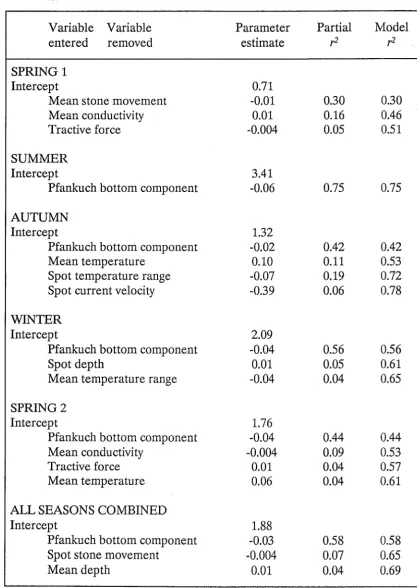
Analysis

Data were analysed with the regression, stepwise regression and Spearman rank correlation procedures of SAS (1985). Stepwise regression of total pigment and epilithic carbon concentration was carried out using the 20 chemical, physical and stability measurements listed in Table 3.1. Concentrations of both total pigment and epilithic carbon were log (x

+

1) transformed prior to this analysis. Spot measurements are those made at the time of collection or in the month prior to the collection of samples. The critical probability for addition and removal of variables to the model was set at 0.05. The same variables were used in the correlation analysis.

RESULTS

Periphyton

Pigment concentrations

Mean total pigment concentrations, for the five stones collected at each site are plotted in Fig. 3.1. Mean maximum biomass at the sites ranged from 15.4 fig

cm-2 _{at Slip Spring to 0.7}_Jig_cm-2 _{at Bruce Stream; mean minimum biomass ranged}

from 4.6 pg cm-2 at Lake Grasmere to Oflg cm-2 _{at several sites. In general, the more}

(44)

16 r'I (\J

I

14 E

0 12 CJ) :::J

10

f-Z

w 8 2: (!)

I-<

6 tl.

-' a::

4

f-0

f-Z

a:: w 2:

ING 2

Figure 3.1. Mean pigment concentrations (n =: 5) on cobbles collected from the study sites between October 1987 and October 1988.

Mean algal biomass (total pigment concentration) decreased logarithmically as overall environmental stability (multivariate stability scores) decreased (F

=

158.24, df = 1,269, P < 0.05, r2

=

0.38) (Fig. 3.2). Mean biomass at the two forest streams fell well below this line, perhaps indicating that light limitation rather than stability was more important to algal communities at these sites. Removal of these two sites from the analysis improved the fit of the model (r2

=

_0.50).

(45)

100~---~

10

1

T

0 0 .l _

T

o

TO

.J. 01

1

O+---,r---+----~---~----+_~~

0.0 0.5 1.0 1.5 2.0 2.5 3.0

MULTIVARIATE STABILITY SCORE

Figure 3.2. Mean periphyton biomass (pigment concentration) at each study site as a function of overall stability (multivariate stability score). Plotted values are averages of the seasonal means ± 1 SE. Regression analysis was performed including seasonal comparisons to yield the equation, loglO (pigment cone.) = 0.76 - 0.34(stability score),,2 = 0.38.

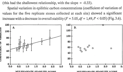
Spatial variation in pigment concentrations (coefficient of variation of values for the five replicate stones collected at each site) (Fig. 3.3) was not related to environmental stability (F

=

2.79, df

=

1,49, P > 0.05). However, as the stability of a site decreased, seasonal variation (coefficient of variation of mean algal bio-mass across the seasons) (Fig. 3.3)