Ellipsometric study on gaseous layers at the solid/water interface

(1)

Author

:

Huseyin Atesci

..

_..

Supervisor

:

Dr

.

ir

.

Herbert Wormeester

Dr

.

J

.

R

.

T

.

Seddon

Physics of Interfaces and Nanomaterials Group

Faculty of Science and Technology

MESA

+

Institute for Nanotechnology

Submitted July 8, 2013

Ellipsometric study on gaseous layers

(2)

i

Abstract

In this thesis, ellipsometry was used to investigate whether gas-enrichment occurs at the solid/water interface, and whether there is a difference in enrichment between hydrophilic and

hydrophobic samples. The samples used were silicon with 277 nm thermal oxide on top (hydrophilic) and an additional silicone oil coating (hydrophobic). The samples were held in a liquid cell which could be filled with degassed, He-saturated, and N2-saturated water. The SiO2 thickness was taken as the fit parameter. Long (>300 minutes) dynamic scans were made on hydrophobic and hydrophilic samples in different water ambients. It was found that it is likely

that gas-enrichment occurs at the solid/water interface due to the qualitative difference

observed in the fitted SiO2 thickness over time between degassed and He-saturated water

ambients. This change was noticeable in the first 150 minutes of measurement and was

observed for both hydrophilic and hydrophobic samples. In the long term, the fitted SiO2 always

increased, which is unlikely to be caused by gas-adsorption through diffusion, but likely to be caused by contaminants. The hydrophilic samples generally showed a larger change in the fitted

SiO2 thickness than the hydrophobic samples. The exact reason why this happens is unclear,

(3)

ii

1. Introduction

For all its importance, water is still not fully understood scientifically. It exhibits in many aspects a different behavior compared to other liquids. One of the aspects where our understanding of water is limited is when water comes into contact with a surface. What really happens with the system at the nanometer scale? Water in its liquid form consists of a very dynamic network of hydrogen bonds, but, when in close contact with a surface, the amount of hydrogen bonds that can be made with the surface determines its hydrophobicity. Hydrophilic surfaces will tend to be terminated with -OH groups which can form hydrogen bonds with water molecules, this will cause water to maximize its contact surface with the hydrophilic substrate. On the other hand, hydrophobic surfaces do not form hydrogen bonds with water, which will cause the network of hydrogen bonds to be disrupted. Water will in turn maximize its contact angle with the surface [1]. It does not end here, however. On hydrophobic substrates, the density of water molecules drops sharply at to the solid/water interface, leading to a depletion layer [2,3-7,8,9]. Gas molecules can fill this depleted zone of water, which is then termed “gas-enriched depletion layer” [10,4,5,7]. Also, additional structures have been discovered recently on substrates that have been wetted: nanobubbles and micropancakes [11-14,15,16,17]. These intriguing topics shall be discussed briefly. It should also be mentioned that what is meant with (nanoscopic) gaseous domains are gas-enriched depletion layers, nanobubbles, and micropancakes. We will first discuss the first aspect.

When a hydrophobic surface is covered with water, the density of water in the direct vicinity of a hydrophobic surface drops sharply. The theoretical groundwork of this

phenomenon was first introduced by Stillinger [18] in 1973. Since then, Barrat et al. investigated

the solid/water interface system with molecular dynamics simulations. They saw a region of depleted density close to the hydrophobic surface of at least one molecule diameter in thickness, with density fluctuations reaching at least 5 molecule diameters into the bulk liquid [19]. Huang et al. performed a molecular dynamics study on a similar system, and found a vapor layer of

approximately 0.3 nm in thickness around hydrophobic objects [20]. Wallqvist et al. have also

observed a vapor layer in a similar research [21]. The thickness of the water vapor layer was

reported to be 0.4 nm for a purely repulsive solid/water interaction. Dammer et al. predicted

that there would be a strong reduction in the density of the Lennard-Jones fluid, which simulated water, near hydrophobic surfaces with density fluctuations with a thickness of as much as 5-10 water molecules [7].

Understanding the physics of the solid/water interface at the nanoscale is important from a fundamental point of view. Hydrophobic spheres in a solution have been used as a simple model to explain phenomena such as protein folding [20]. Understanding depletion layers, whether they are filled with gas or not, is critical for explaining chemical reactions in a liquid at the solid/water interface. It has also consequences for our understanding of slip boundary conditions of water at the substrate surface [21]. This topic is often connected to the very recent discovery of nanobubbles and micropancakes.

(5)

2

with a water density of only 9% of that of bulk water, although that could be caused by air trapped (nanobubbles) at the solid/water interface [8]. Again using neutron reflectometry, Doshi et al. found a reduced density layer of water in the direct vicinity of the hydrophobic substrate [5]. Furthermore, they found that the thickness of the depletion layer depended on whether the water contained dissolved gases. When ambient water was used to cover the hydrophobic substrate, the depletion layer had a thickness of 1.1 nm, while argon-gassed water

showed a depletion layer of 0.2 nm. Also, studies made by Dammer et al. [7] and others [4] show

that it is highly likely that there is a gas-enriched depletion layer at the direct vicinity of the hydrophobic substrate. However, there seems to be no consensus in the scientific community on whether gas-enriched depletion layers exist [6]. In general, the scientific publications show results in favor of a depletion layer, with a typical thickness that can range from 0.1 nm to approximately 1 nm [2,3,8,9].

On the other hand, experiments have also been made about which the authors have stated that the depletion layer is either unlikely to happen or that they are inconclusive about it.

For example, Jensen et al., were unable to distinguish quantitatively the depletion layer of water

on a hydrophobic surface using X-ray reflectometry, possibly due to low contrast between water and the substrate. They state that if the depletion layer does exist, the density of water at the depletion layer is approximately 90% of that of bulk water with a thickness of 0.1 nm [22]. Ellipsometry studies that have been published thus far generally belong to this area of opinion. Ellipsometry is a widely used tool for thin-film characterization. It is non-destructive, has a fast time resolution, and does not require delicate vacuum systems or low temperatures. Ellipsometry measures density variations at the solid/liquid interface. However, it has a poor lateral resolution, and cannot distinguish between nanobubbles, micropancakes, or gas-enriched depletion layers, just like X-ray reflectometry and neutron reflectometry. It is, however, suited

for determining whether gas enrichment occurs at the solid/water interface. Castro et al., for

example, have observed a layer of air of 0.5-1.0 nm in the depletion layer on a polystyrene layer of approximately 65 nm thick [10]. However, they did not see any air layer for a thicker layer of

polystyrene of approximately 300 nm. Mao et al. investigated water on hydrophobic agents, they

concluded that, if there were to be a layer of air in the depletion layer, it should be less than 0.1 nm thick [23]. Takata et al. stated that they found no evidence of a depletion layer [21]. The substrate they used was a hydrophobic alkylsilane in water.

It should be noted that X-ray reflectometry, neutron reflectometry, and ellipsometry cannot distinguish between gas-enriched depletion layers, or a high density of nanobubbles or micropancakes.

We will now focus shortly on these two forms of gaseous domains that can appear in a wetted surface: nanobubbles and micropancakes.

When pouring water in a glass beaker, one can clearly see the glass surface being wetted

after the macroscopic bubbles have dissolved. However, when zoomed-in on a microscopic level, one would still observe miniscule gaseous domains at the solid/water interface. These microscopic gaseous domains exist in two main forms: nanobubbles [11,12,14-16] and

micropancakes [13,17]. Nanobubbles were first reported in the literature by Parker et al. [14]

(6)

3

that nanobubbles smaller than 100 nm in size would fill the gap between the plates and cause an increase in the attractive force between them. The statement was a controversial one, because it was widely accepted that gaseous domains submerged in a liquid with dimensions measured in nanometers could not be stable, due to the gas inside the bubble rapidly dissolving into the surrounding liquid. This is the classical prediction by the Laplace equation [24]. Currently, the hydrophobic attraction is understood as capillary forces that arise when nanobubbles bridge the two hydrophobic plates.

A multitude of experimental techniques have been used to investigate surface nanobubbles, such as internal reflection infrared spectroscopy [25], rapid cryofixation [26], neutron reflectometry [16], and X-ray reflectometry [27]. Due to its excellent spatial resolution, unlike the methods mentioned before, the atomic force microscope (AFM) is usually preferred for surface nanobubble investigation [28,29].

In the experiments that have been done until recently, surface nanobubbles have been found with typical heights of 10-20 nm and widths of 50-100 nm with a spherically-capped shape. Micropancakes are much wider – several microns in diameter, but only 1-2 nm in height [6]. Nanobubbles have been found to be stable in water for days [30], outlasting classical lifetime predictions by at least 10 orders of magnitude. Why the classical prediction fails and nanobubbles are stable is not clearly understood and is a topic of debate.

The connection between (gas-enriched) depletion layers and nanobubbles and micropancakes is not always clear. There is a difference between nanobubbles and gas-enriched depletion layers in that they have different appearances. On the other hand, micropancakes are possibly related to the gas-enriched depletion layers [6]. It might be that all three types of gaseous domains are present on the surface when a hydrophobic substrate is submerged in water. Apart from the fact that there is no clear answer why nanobubbles are stable, there is also no consensus of the scientific community whether there is a gas-enriched depletion layer at all.

This thesis will focus on trying to answer the question following questions:

1) Does gas enrich the solid/water interface?

2) Is there a difference in enrichment between hydrophobic and hydrophilic surfaces?

We will use ellipsometry as our main experimental technique to qualitatively (and where possible, quantitatively) analyze whether gas layers form on the surface. The substrates that will be used are silicon with both a native oxide and thick oxide layer on top. The liquid used in our case is ultrapure Milli-Q water, with the option that it can be degassed or gas-saturated with a specific gas type. The silicon samples will also be hydrophobized to see the difference between hydrophilic and hydrophobic interfaces and whether gaseous domains form more easily at the latter. The effects of different gas types dissolved in water will also be investigated.

The conclusions of the previously performed ellipsometry by Mao et al. [23], Takata et al.

[21], and Castro et al. [10], lean towards the statement that gaseous domains at the solid/water

(7)

4

Bibliography of Introduction

1. Torigoe, A.D.How water meets a hydrophobic surface: Reluctantly and with fluctuations. s.l. : University of Illinois,

2006.

2. On the origin of the hydrophobic water gap: An X-ray reflectivity and MD simulation study. M. Mezger, F. Sedlmeier,

D. Horinek, H. Reichert, D. Pontoni, H. Dosch. 6735-6741, s.l. : Journal of the American Chemical Society, 2010, Vol.

132.

3. How water meets a hydrophobic surface. A. Poynor, L. Hong, I.K. Robinson, S. Granick. 266101, s.l. : PRL, 2006, Vol.

97.

4. Interfacial water at hydrophobic and hydrophilic surfaces: Slip, viscosity, and diffusion. C. Sendner, D. Horinek, L.

Bocquet, R.R. Netz. 10768-10781, s.l. : Langmuir, 2009, Vol. 25.

5. D.A. Doshi, E.B. Watkins, J.N. Israelachvili, J. Majewski. 9458, s.l. : Proceedings of the National Academy of

Science, 2005, Vol. 102.

6. Nanobubbles and micropancakes: Gaseous domains on immersed substrates. J.R.T. Seddon, D. Lohse. 133001, s.l. :

Journal of Physics: Condensed Matter, 2011, Vol. 23.

7. Gas enrichment at liquid-wall interfaces. S.M. Dammer, D. Lohse. 206101, s.l. : PRL, 2006, Vol. 96.

8. Interaction of water with self-assembled monolayers: Neutron reflectivity measurements of the water density in the

interfaces region. D. Schwendel, T. Hayashi, R. Dahint, A. Pertsin, M. Grunze, R. Steitz, F. Schreiber. 2284-2293,

s.l. : Langmuir, 2003, Vol. 19.

9. Water and ice in contact with octadecyl-trichlorosilane functionalized surfaces: A high resolution X-ray reflectivity

study. M. Mezger, S. Schöder, H. Reichert, H. Schröder, J. Okasinski, V. Honkimäki, J. Ralston, J. Bilgram, R. Roth,

H. Dosch. 244705, s.l. : Journal of Chemical Physics, 2008, Vol. 128.

10. L.B.R. Castro, A.T. Almeida, D.F.S. Petri. 7610, s.l. : Langmuir, 2004, Vol. 20.

11. Images of nanobubbles on hydrophobic surfaces and their interactinos. J.W.G. Tyrrell, P. Attard. 176194, s.l. : PRL,

2001, Vol. 87.

12. Nanobubble trouble on gold surfaces. M. Holmberg, A. Kühle, J. Garnaes, K.A. Morch, A. Boisen. 10510-3, s.l. :

Langmuir, 2003, Vol. 19.

13. Nanoscale multiple gaseous layers on a hydrophobic surface. L. Zhang, X. Zhang, C. Fan, Y. Zhang, J. Hu. 8860-4,

s.l. : Lanmguir, 2009, Vol. 25.

14. Bubbles, cavities and the long-ranged attraction between hydrophobic surfaces. J.L. Parker, P.M. Claesson, P.

Attard. 8468-8480, s.l. : Journal of Physical Chemistry, 1994, Vol. 98.

15. Nanobubbles on solid surface imaged by atomic force microscopy. S. Lou, Z. Ouyang, Y. Zhang, X. Li, J. Hu, M. Li, F.

Yang. 2573-5, s.l. : Journal of Vacuum Science & Technology B, 2000, Vol. 18.

16. Nanobubbles and their precurson layer at the interface of water against a hydrophobic substrate. R. Steitz, T.

Gutberlet, T. Hauss, B. Klosgen, R. Krastev, S. Schemmel, A.C. Simonsen, G.H. Findenegg. 2409-2418, s.l. :

Langmuir, 2003, Vol. 19.

17. Detection of novel gaseous states at the highly oriented pyrolytic graphite-water interface. X.H. Zhang, X. Zhang, J.

Sun, Z. Zhang, G. Li, H. Fang, X. Xiao, X. Zeng, J. Hu. 1778-83, s.l. : Langmuir, 2007, Vol. 23.

18. Stillinger, F.H. 141, s.l. : Journal of Solution Chemistry, 1973, Vol. 2.

19. Barrat, J. L. and Bocquet, L. 4671, s.l. : PRL, 1999, Vol. 82 (23).

20. J. Janacek et al. 8417-8429, s.l. : Langmuir, 2007, Vol. 23.

(8)

5

22. T.R. Jensen, M.O. Jensen, N. Reitzel, K. Balashev, G.H. Peters, K. Kjaer, T. Bjørnholm. 086101-1, s.l. : PRL, 2003,

Vol. 90 (8).

23. M. Mao, J. Zhang, R.H. Yoon, W.A. Ducker. 1843, s.l. : Langmuir, 2004, Vol. 20.

24. V. Stuart, J. Craig. 40-48, s.l. : Soft Matter, 2011, Vol. 7.

25. Nanobubbles at the interface between water and a hydrophobic solid. X.H. Zhang, A. Quinn, W.A. Ducker.

4756-4764, s.l. : Langmuir, 2008, Vol. 24.

26. Rapid cryofixation/freeze fracture for the study of nanobubbles at solid-liquid interfaces. M. Switkes, J.W. Ruberti.

4759, s.l. : Applied Physics Letters, 2004, Vol. 84.

27. High-resolution in situ X-ray study of the hydrophobic gap at the water-octadecyl-trichlorosilane interface. M.

Mezger, H. Reichert, S. Schoder, J. Okasinski, H. Schroder, H. Dosch, D. Palms, J. Ralston, V. Honkimaki.

18401-18404, s.l. : PNAS USA, 2006, Vol. 103.

28. Boundary slip and nanobubble study in micro/nanofluidics using atomic force microscopy . Y. Wang, B. Bhushan.

29-66, s.l. : Soft Matter, 2010, Vol. 6.

29. M. Mazumder, B. Bhushan. 9184-9196, s.l. : Soft Matter, 2011, Vol. 7.

30. Correlation between geometry and nanobubble distribution on HOPG surface. S. Yang, E.S. Kooij, B. Poelsema, D.

(9)

6

2. Methodology

Following up on the goals of this thesis set in the Introduction, several theoretical and experimental aspects are mentioned in this chapter to give the reader an understanding of the research done by the author. Firstly, the sample preparation and measuring methods will be explained. Ellipsometry and our experimental setup will be discussed next, followed by the modeling methods used.

2.1 Sample preparation

Due to the scope of research that can be done on this area, there is a limited selection of base substrates to see whether gas-enriched depletion layers form. These are (i) silicon with native oxide (1-2 nm) and (ii) thermal oxide (277 nm) on top. Native silicon oxide is the oxide layer which forms on silicon when it is exposed to air, while thermal silicon oxide can be grown on silicon when it is heated in the presence of oxygen. The silicon oxide top layer has a highly hydrophilic property. However, this is only the case when it is freshly cleaned, because silicon is quickly contaminated with (organic) particles, which increases its hydrophobicity. When coated with a hydrophobic organic layer, it will exhibit a hydrophobic property.

2.1.1 Hydrophilic samples

The method used to acquire hydrophilic silicon samples is applicable for both native and thick oxide silicon. Silicon samples are first diced in approximately 15 15 mm-sized squares with a thickness of 0.5 mm. After this process, the samples are put in a glass beaker and cleaned with a piranha solution (a mixture of H2SO4 and H2O2 in a 3:1 volume ratio). This treatment will remove organic material from the surface and the sample will be ready for measurement after it is rinsed with Milli-Q water several times.

2.1.2 Hydrophobic samples

(10)

7

2.1.3 Vapor coating

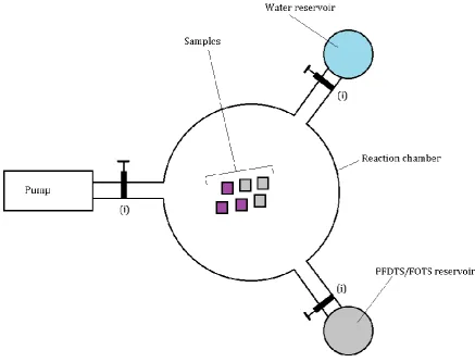
Vapor coating with FOTS or PFDTS requires a chamber with several attachments that can

[image:10.595.81.519.151.484.2]

be put under low pressure, a schematic overview of which can be seen in Figure 1.

Figure 1. Schematic top view of the reaction chamber used to coat samples with PFDTS and FOTS. The valves are

denoted by (i).

The samples are put in the main reaction chamber, which is put under low pressure

(usually around 5 10-2_{mbar) with a pump. There are two attachments with a valve to the main}

(11)

8

2.1.4 Silicone oil coating

After the silicon samples are cleaned in the plasma chamber, silicone oil is applied immediately on its surfaces, covering it completely. Then the samples are put in a UV chamber where they are irradiated for 10 hours. This is the step where the silicone oil molecules are broken down and chemically bind with the substrate interface, as explained in section 5.1.3. Hereafter, the samples are put in a beaker in a sample holder in a mixture of iso-octane and acetone in a 1:1 volume ratio while stirring. This step washes off the oil and takes about 30 minutes. Then the liquid is replaced by acetone and is followed by another 30 minutes stirring period. The samples are then rinsed with deionized water and put in an oven at 120 °C for one hour in a vacuum environment to prevent contamination. This is the final step and the samples are ready for measurement.

2.2 Contact angle measurements

Differentiating between hydrophilic and hydrophobic surfaces is an important aspect in this thesis. One of the ways to do this is to use an optical contact angle measurement. Static contact angle measurements usually are sufficient for this purpose.

2.2.1 Static contact angle

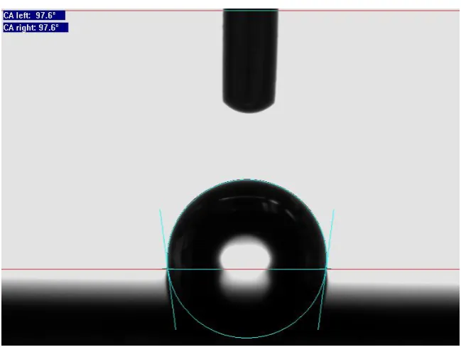
[image:11.595.136.461.490.734.2]

Measuring the static optical contact angle will provide information about the hydrophobicity of the surface. If the static contact angle exceeds 90°, the surface is classified as hydrophobic. If it is below 90°, it will be classified as hydrophilic. The measurement procedure with the goniometer is as follows: the sample is set on a flat surface where it is in view of the camera. A syringe infuses a Milli-Q water drop of 1 μL on the surface, the curvature of the droplet is then analyzed by the program. The angle between the droplet surface and the flat surface is drawn and calculated, as it can be seen in Figure 2.

(12)

9

2.3 Ellipsometry

The main measuring technique used in this thesis to research potential gas-saturated layers forming on the solid/water interface, is ellipsometry.

Ellipsometry has been known since 1887, when Drude formalized its equations [1]. Ellipsometry measurements were initially conducted at a single wavelength of light and were time consuming. In the late 20th_{century, the process became automatized [2] and it quickly grew to} being a common method for studying thin film layers. The following section briefly discusses the basics of ellipsometry.

2.3.1 Basics of ellipsometry

Light is a propagating electromagnetic wave traveling at light speed . It has an

oscillating transverse electric and magnetic field, but, for the purposes of this paper, it is sufficient to look only at the oscillating electric field.

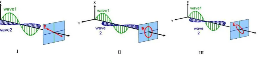
[image:12.595.74.527.369.472.2]

When light is emitted from a regular light source, like a lamp, its electric fields orient randomly in all possible directions perpendicular to the propagation vector [3]. This is referred to as unpolarized light. Next to this, there are several forms of polarization of light: linear, circular, and elliptical. These can be seen in Figure 3.

Figure 3. Polarization of light in three different forms: linear (I), circular (II), and elliptical (III). Wave 1 and 2 indicate

the electric field oscillations of the s and p components of the electrical field [7].

When the electrical field is oscillating perpendicularly in one plane, it is linearly polarized. When the endpoint of the electrical field intensity precesses along a circular and elliptical trajectory, it is referred to as circular and elliptical polarized light, respectively. The time needed for one precession is defined as , where is the angular frequency of light [4].

2.3.2 Parameterization

The polarization of the electrical waves of light is parameterized into the s and p

polarizations. The s and p polarization refer to the component of the electrical field

(13)

[image:13.595.159.446.73.356.2]

10

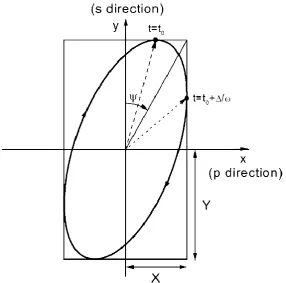
Figure 4. Theprecession of the electrical field of a light wave as seen from the direction of its propagation [4].

When light with a known polarization is reflected off a surface, its polarization will

change as can be seen in Figure 5. The interpretation of and is discussed later on in this

section.

Figure 5. Linearly polarized light which reflects off a surface acquires a polarization change. In this case the reflected

[image:13.595.73.517.465.697.2]

(14)

11

This change in polarization is determined for example by the angle of incidence, and the optical properties of the surface, such as film thickness, roughness, dielectric constants, etc. The

change in polarization is expressed by two main parameters: and . The parameter refers

to the ratio of reflection coefficients of the s and p polarized light waves:

The parameter refers to the phase difference between the s and p polarized light waves:

The and denote the phase change acquired by the s and p polarized light waves respectively upon reflection from the surface. In ellipsometry, the complex reflectance ratio [6] is measured, which is the ratio between the s and p reflection coefficients, and is given commonly expressed as:

It is for this reason that ellipsometry is relatively insensitive to intensity fluctuations and requires no reference beam. Furthermore, it is a highly accurate and reproducible measuring method, with a thickness sensitivity that can reach ~0.1 Å [6].

2.3.3 Modeling

(15)

[image:15.595.125.466.73.284.2]

12

Figure 6. Modeling procedure for ellipsometry data [7].

An important remark would be that one can adjust any parameter in a model and still match the ellipsometry data nicely, while it would not have any physical meaning. This is why it is important to keep the number of fit parameters as low as possible.

2.3.4 Advantages and disadvantages

The main advantages of ellipsometry are that it is non-destructive, highly accurate. However, ellipsometry has a very low spatial resolution. It is an indirect method because of the necessity of an optical model for data analysis. Furthermore, ellipsometry data have to be supported by other characterization methods such as Atomic Force Microscopy (AFM), to gain a proper understanding of the topology of the surface that is under investigation [6].

2.3.5 Further reading

For the reader who is interested in reading an in-depth theoretical background on ellipsometry, books by H. Fujiwara [6], H. G. Tompkins [3,4] are good choices.

2.4 Experimental setup

(16)

[image:16.595.81.515.82.315.2]

13

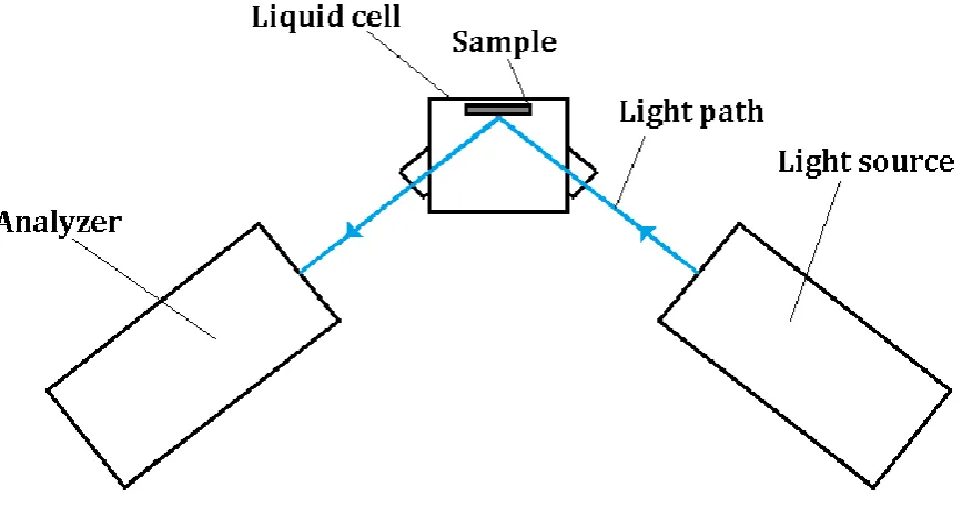
Figure 7. Schematic top view of the ellipsometry setup with the water-filled liquid cell mounted.

When measuring the effect of a degassed or gas-saturated (with an arbitrary gas type) water ambient, the sample is submerged in water and light from the source reflects off it. The reader should note that the system in the liquid cell is not closed, thus when the gas type dissolved in the liquid is not equal to that of air, diffusion will take place and is noticeable after typically 30 minutes with the oximeter (this in turn depends on how long the diffusion length is).

2.4.1 Spectroscopic scans and dynamic scans with the ellipsometer

The experiments done with the ellipsometer are done in two ways: spectroscopic scans and dynamic scans. The methods of performing each type of scan will be discussed below.

Before any measurement is done, there is a standard procedure of degassing the entire liquid cell with sample mounted, and Milli-Q water filling it. The liquid cell is placed in an evacuation chamber, which is connected to a membrane pump. The chamber is then depressurized, this is done to remove any gaseous domains on the surface of the substrate. The

degassing procedure inside the evacuation chamber lowers the O2 concentration in water to less

than 1% of that of its saturation value. It is assumed the other gases naturally present in water

will also be largely removed, even though we only recorded the O2 saturation. While degassing

the water in the liquid cell, the temperature drops as a result of water evaporating, that is why a heater is held underneath the chamber to keep the water in the liquid cell at room temperature. This step takes approximately 25 minutes, after which the entire liquid cell is removed from the evacuation chamber, and mounted for measurement. The first scan is interpreted as a control measurement.

Gas-saturated water is prepared by degassing water in an evacuation chamber for approximately 15 minutes, whilst stirring and at room temperature. Hereafter, a saturator is

(17)

14

The preparation of gas-saturated water is then complete and can be used to change the water ambient in the liquid cell explained in 2.4.2.

2.4.2 Spectroscopic scans

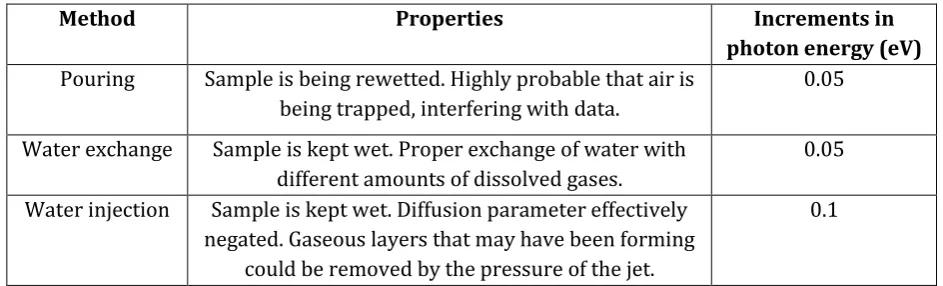
To negate the effects of diffusion, spectroscopic scans would have to take less than 30 minutes to complete. In our case spectroscopic scans usually take approximately 25 minutes, with increments in the photon energy of 0.05 eV. One could measure for a shorter period of time, but the energy resolution would deteriorate.

The reader should be reminded that the ellipsometer data is gathered from a patch of light of several mm2_{that is reflected off the sample. To compare the effects of gas-saturated} water compared to degassed water, one would have to repeatedly change the water ambient between degassed and gas-saturated water. The different ways to cycle between gas-saturated and degassed water ambients is explained in the following:

 The first method is simply to empty the liquid cell of the bulk of its water with a syringe,

after which a freshly prepared amount of water is poured in the cell. For example, if the liquid cell has degassed water, after the measurement it is removed and replaced with gas-saturated water, then with gas-saturated water, etc. One clear disadvantage of this method is that the sample becomes dry when removing the water from the liquid cell, and air may get trapped to form nanobubbles at the surface. What would then be measured is not any surface-induced gas on the substrate surface, so the results taken with this method could be misleading. It is also not straightforward to have a consistent way of pouring water in the liquid cell.

 The second filling method is by exchanging the water while it is mounted. After

(18)

[image:18.595.72.526.68.412.2]

15

Figure 8. Photo taken of the liquid cell after measurement with the exchange method.

 The third method relies on injecting the liquid directly on the light spot where data is

(19)

[image:19.595.73.527.84.426.2]

16

Figure 9. Photo taken of the liquid cell with the water injection tube mounted. Note that the liquid cell is dry in this

case.

During the entire period of each measurement, water is injected onto the sample. This would mean that the local environment near the surface becomes changed instantly and one would not have to rely on diffusion of gas. It also possible that any gaseous layer that may be forming at the solid/water interface could be removed by the pressure of the water jet. At each measuring cycle, the water reservoir which feeds the injection tube is changed. Due to the limited amount of water in the syringe (100 mL), which is connected to the syringe pump, the measuring time is restricted to about 12 minutes. This in turn means that the increments made in the photon energy should be 0.1 eV.

(20)

17

Method Properties Increments in

photon energy (eV)

Pouring Sample is being rewetted. Highly probable that air is

being trapped, interfering with data.

0.05

Water exchange Sample is kept wet. Proper exchange of water with

different amounts of dissolved gases.

0.05

Water injection Sample is kept wet. Diffusion parameter effectively

negated. Gaseous layers that may have been forming could be removed by the pressure of the jet.

[image:20.595.62.534.69.212.2]

0.1

Table 1. Properties of each measuring method listed together with the energy increments (which indicates energy

resolution) made during measurement.

2.4.3 Dynamic scans

Dynamic scans, which are series of spectroscopic scans, may take a lot longer to include the effect of diffusion, and hence possible gas adsorption, in the ellipsometer signal. Usually they take longer than 100 minutes. The experimental procedure is the same as explained under section 2.4.1: the liquid cell with sample placed and degassed water inside, is mounted on the ellipsometer for measurement. This is the main starting point for all dynamic scans.

From this point on, if the measurement has to be done in a degassed water ambient, the water is not exchanged with another water type, so air will diffuse in the water and onto the sample, which can then be related to the difference in ellipsometer signal measured.

For initial N2-saturated and He-saturated water ambients, the degassed water is simply

exchanged by N2-saturated and He-saturated water, and the measurements start immediately

after the exchange process.

2.4.4 Sample cleaning

Due to the limited amount of samples compared to the larger amount of experiments done, it is important to consistently clean samples. Hydrophobic and hydrophilic samples have their own method of doing so.

 After each measurement, hydrophobic samples undergo cleaning in an ultrasonic bath in

a hexane solution for 15 minutes. Here after, the hexane is replaced by acetone and the process is repeated. Then, the samples are rinsed in Milli-Q water 5 times, after which the cleaning procedure is completed. The samples are stored in air.

 Hydrophilic samples are cleaned using piranha, after which they are rinsed 10 times in

Milli-Q water. This completes the cleaning procedure and the samples are stored in air.

2.5 Diffusion of gas in water

(21)

18

calculated gas saturation profile can be used to fit and subsequently plot the change in ellipsometer signal against the gas concentration in the BET model.

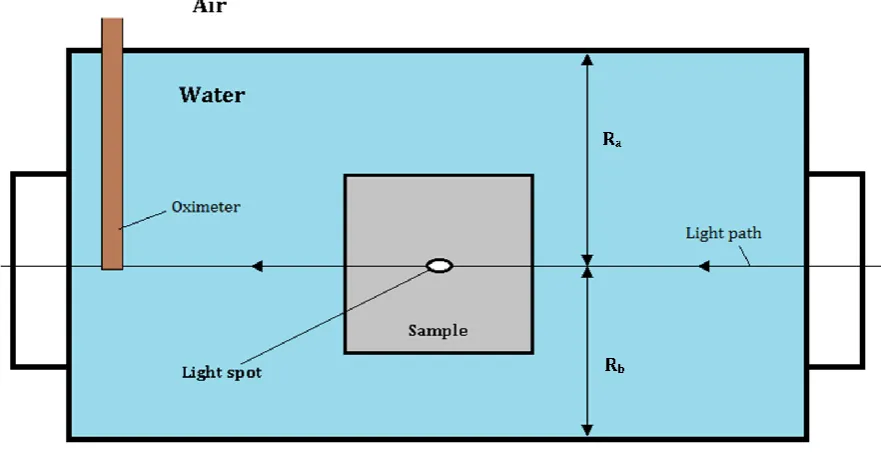
[image:21.595.81.522.198.424.2]

Diffusion of gas in water in the vertical direction is similar to heat diffusion. Fick’s second law of diffusion will be used in our case to relate the concentration of gas near the light spot on the sample to the time, as can be seen in Figure 10.

Figure 10. Schematic front view of the liquid cell during measurement.

For future calculations, we define a location variable inside the liquid cell R as:

The main equation used to find an expression for the concentration of gas u(x,t) (mol/m3_{) as a function of depth}_x_{(m) and time}_t_{(min) is given below:}

D is the diffusion constant of a type of gas in water (m2_{/s), it can range from 1 to 7} ₁₀-9

m2_{/s depending on the molar volume of the type of gas [8]. High molar volume gas types (such}

as CH3Br) show a diffusion constant between 1 and 2 10-9 m2/s at 25 °C. Low molar volume gas

types (such as He) show a diffusion constant higher than 3 10-9 _m2_{/s. In our case, diffusion} constants of O2 and N2 are similar: 2 10-9 and 1.9 10-9 m2/s at 25°C, respectively [9]. The steady state solution for the concentration profile us(x) is a constant uout, which is the saturation concentration of any arbitrary type of gas in water.

(22)

19

v(x,t) represents the difference between the time dependent solution and the steady state solution. When identifying the boundary conditions for v(x,t), one can arrive at the following:

The depth x ranges from 0 to L, with 0 being the water/air interface at the top and L the bottom of the liquid cell. After separation of variables and solving the time and space dependent differential equations separately, we arrive at the following:

The concentration profile u(x,t) is a summation which is dependent on the amount of Fourier coefficients n (which, for computational reasons will be finite) and coefficient bn. The starting concentration of gas in the liquid cell is not zero, but a value u0.

2.6 BET-model

The BET-model is often used for explaining the adsorption of gas molecules at a solid surface. The BET equation is as follows:

Where p is the pressure (N/m2) of the gas, p₀is the saturation pressure of the gas, v is the

volume of the gas adsorbate on the surface, vmis the volume of one monolayer of gas adsorbate,

and c is the BET constant which is related to the energy of adsorption and liquefaction of the gas

[13]. This model can be used to see if our data can be fitted with the BET theory, and whether the gas pressure plays a role in the thickness of a possible gas adsorbate layer.

2.7 Model predictions

(23)

20

2.7.1 Effect of dissolved air in water

The effect of air dissolving in water could be affecting ellipsometry data by changing the refractive index of water. To investigate if such an effect is playing a significant role in our system, the Lorentz-Lorenz equation is used which relates the polarizability of a material to its refractive index. Table 2 contains the necessary information to calculate the change in refractive index of pure, degassed water as it is gassed with air in a steady state solution.

Molecule type Polarizability volume (Å3₎ [10,11]

Amount of particles in steady state 1 mol water solution (mol) [12]

H2O 1.45 1

N2 1.76 1.1 10-5

O2 1.56 2.34 10-5

CO2 2.56 6.12 10-4

Table 2. Polarizability volumes (Å3_{) and amount of particles of gas dissolved (mol) in 1 mol water at the steady state}

solution given for several molecule types.

The polarizability volume can easily be converted to the molecular polarizability in SI units by multiplying with 1/4πε0. The total polarizability is given by the following formula:

When comparing the total polarizability of air gassed water to that of pure, degassed

water ( ), it has increased with 0.047%.

This change in polarizability would translate to a maximum difference in refractive index

of less than 3.5 10-8_{% compared to the pure water ambient. This is calculated with the}

Lorentz-Lorenz equation:

With n being the refractive index, N the number of molecules in the given volume, and α

the mean polarizability in Cm2_V-1_.

Thus it can be argued that the change in refractive index due to dissolved gases would not be influencing the ellipsometer signal, because the effect will be dominated by signal noise.

2.7.2 Modeling with WVASE software

(24)

[image:24.595.127.473.85.213.2]

21

Figure 11. Schematic overview of the most common model used in this thesis. The first layer (i) is the Si substrate

with a thickness of 1 mm. (ii) is the mixing layer between Si and SiO2, which is always set to 0.05 nm. (iii) is the SiO2

layer, which will include the following: SiO2, organic hydrophobic coating, gas adsorbates, or even contaminations.

The thickness of this layer is the fitting parameter. The final layer (iv) is the water ambient, the temperature of which is 21 ± 1°C, and can be assumed constant.

In this case, the only fit parameter is the SiO2 thickness. It was a deliberate choice not to include extra layers for the hydrophobic organic coating and potential gas-enriched depletion layers to keep the number of parameters at a minimum. The thickness of the solid substrate (i.e.

SiO2 and, if used, the hydrophobic organic coating) is assumed to be constant. The change in the

fitted thickness of the SiO2 layer could then be attributed to gaseous bodies forming at the solid/water interface (note that this method cannot distinguish between nanobubbles or gas adsorbates, as explained before). One could use the equation for the optical thickness [14] to relate the real average thickness of a layer , to its refractive index and fitted thickness

:

The problem when calculating with this method is that and are unknown to begin

with. We would then increase the number of parameters for our fit, which is undesirable. Even if

we would only use the SiO2 thickness as a fitting parameter, this would not defeat the purpose of

this thesis. After all, it is the qualitative differences in ellipsometer signals between different samples and conditions we are looking for.

2.7.3 Modeling with WVASE software prior to measurement

The system under investigation has a number of variables that have an effect on our

ellipsometer signal. These are for example: the temperature, the SiO2 layer thickness, changes in

(25)

22

Bibliography of Methodology

1. Ueber die Gesetze der Reflexion. Drude, P. 12, s.l. : Annalen der Physik, 1889, Vol. 268.

2. D.E. Aspnes, A.A. Studna. 220-228, s.l. : Applied Optics, 1975, Vol. 14.

3. Tompkins, H.G.A User's Guide to Ellipsometry. 1993.

4. H.G. Tompkins, E.A. Irene.Handbook of ellipsometry. 2005.

5. University of Dublin. [Online] http://www.tcd.ie/Physics/Surfaces/ellipsometry2.php.

6. Fujiwara, H.Spectroscopic ellipsometry principles and applications. s.l. : John Wiley & Sons, 2007.

7. [Online] J.A. Woollam Co., Inc. http://www.jawoollam.com/tutorial_5.html.

8. Uncertainties in the Molecular Diffusion Coefficient of Gases in Water for Use in the Estimation of Air-Sea Exchange.

D.B. King, W.J. De Bruyn, M. Zheng, E.S. Saltzman. s.l. : University of Miami, 1995.

9. Cussler, E.L.Diffusion - mass transfer in fluid systems. Cambridge : Cambridge University Press, 1984.

10. Molecular and Atomic Polarizabilities: Thole's Model Revisited. P.T. Duijnen, M. Swart. 14, s.l. : Journal of Physical

Chemistry A, 1998, Vol. 102.

11. Pauling, L.General Chemistry. s.l. : Courier Dover Publications, 1988.

12. Sander, Rolf. Henry's Law. [Online] http://www.henrys-law.org/.

13. S. Brunauer, P.H. Emmett, E. Teller. 309, s.l. : Journal of the Americal Chemical Society, 1938, Vol. 60.

(26)

23

3. Results and discussion

The analyzed data gathered in the course of this thesis, together with the discussion thereof, will be summed up in this section. Firstly, the contact angle data on the samples that were prepared will be presented. Secondly, we will look at the results obtained by the dynamic scans and how to interpret them with the oxygen diffusion data and the BET theory. Further on in this chapter, recommendations have been proposed for future experiments to gain a more thorough understanding on this subject.

3.1 Contact angle measurements on prepared samples

Two main substrates were investigated in this thesis: silicon with thermal oxide (277 nm), and silicon with native oxide (1-2 nm) on top. Due to the time limitations, our attention was focused more heavily on the thermal oxide silicon than the native oxide samples. Both substrate types are by themselves hydrophilic due of the –OH terminated groups at the interface. The static contact angle of freshly etched silicon oxide (i.e. non-coated) samples typically has values of 5°.

(27)

24

Coating type Average static contact angle before H2O wetting

(°)

Average static contact angle after

H2O wetting (°)

RMS roughness (nm)

FOTS 105.0 ± 1.5 103.6 ± 1.5 Not measured

Silicone oil 96.9 ± 1.5 97.7 ± 1.5 0.71

PFDTS 95.2 ± 1.5 90.1 ± 1.5 Not measured

[image:27.595.66.532.333.440.2]

No coating 5.0 ± 1.5 Not measured1 _0.23

Table 3. The average static contact angle before and after 91 hours of wetting with H2O for different coating types.

The RMS roughness is also included.

In the second case, the effects of wetting in the IPA/acetone mixture was tested, as these samples undergo cleaning with these chemicals. The total wetting time was 5 hours, and the results can be seen in Table 4.

Coating type Average static contact angle before IPA/acetone cleaning

(°)

Average static contact angle after IPA/acetone cleaning

(°)

FOTS 105.0 ± 1.5 96.0 ± 2.0

Silicone oil 96.9 ± 1.5 96.3 ± 1.5

Table 4. The average static contact angle of FOTS and Si oil samples before and after IPA/acetone cleaning.

From these results it can be seen that from all hydrophobic coating types, the static contact angle for PFDTS dropped considerably after the wetting period in water. The static contact angle for FOTS and silicone oil remained the same within the error margin. It is because of this result that the PFDTS was not used as a coating type in our measurements performed in the liquid cell, because a change in the ellipsometry signal could be attributed to the effects related to the observed static contact angle decrease upon extended contact with water. Furthermore, it is observed that FOTS coatings are affected by the IPA/acetone mixture. When taking all these results in consideration, Silicone oil was the most used chemical for hydrophobization, not only due to its resilience to chemical cleaning, as stated by Arayanarakool et al. [1], but also due to the relative ease with which it can be made.

3.2 Dynamic scans

During the course of this thesis, several experimental techniques have been tried to test our hypothesis. It was found out eventually that in our case, there are a number of parameters

(28)

25

that cannot be controlled fully, such as air diffusing in our water-filled liquid cell, or the oxygen (or other gases) concentration at the start of the measurement. Therefore, any other parameters were controlled as much as possible, as explained in section 2.4.3 and 2.4.4 of the Methodology. The dynamic scans were done on both hydrophilic uncoated and silicone oil coated samples in water ambients that differed in their initial compositions of gas. This set of experiments is listed in Table 5.

Sample type Initial composition of ambient

Uncoated silicon oxide (hydrophilic) Degassed water

N2 saturated water He saturated water

Silicone oil coated silicon oxide (hydrophobic) Degassed water

N2 saturated water He saturated water

Table 5. The measurement setup used for the dynamic scans.

After each dynamic scan, the ellipsometry data is fitted with the models using the WVASE

software. The fitting parameter was the SiO2 thickness, which as described before is a parameter

used to describe change at the solid/water interface. Each dynamic scan is comprised out of a multitude of spectroscopic scans that take 25 minutes. The very first spectroscopic scan is set as the baseline measurement, with a certain fitted SiO2 thickness. The spectroscopic scans that

follow it are analyzed, and the fitted SiO2 thicknesses are subtracted from the SiO2 thickness of

the initial scan. The result is a normalized fitted SiO2 thickness curve plotted against the time.

(29)

[image:29.595.54.546.75.700.2]

26

Figure 12. The analyzed measurements from the dynamic scans where data is plotted as the normalized fitted SiO2

thickness (nm) against the time (min). The graphs in (i), (iii), and (v), show the curves for the hydrophilic samples, situated in a He-saturated, degassed, and N2-saturated ambient, respectively. The graphs in (ii), (iv), and (vi), show the

(30)

27

It should be noted that not all the scans have been done three times due to the time limitations. Nonetheless it is possible to discuss the current results. The following section will

discuss the graphs depicted in Figure 12.

1) Growth curves for the degassed water ambient tend to increase at a fast rate at the start

[image:30.595.158.466.179.426.2]

of the measurement, and slow down until a saturation point is reached, typically after more than 3000 minutes of measurement. See also Figure 13.

Figure 13. The normalized fitted SiO2 thickness curve for a long (>3000 minutes) dynamic scan. The

measurement was in this case the 1st_{Hydrophobic – Degassed scan.}

2) In the He-saturated water ambient, the growth curve at the start is different: there is an

initial time period where there is no growth, or a reduction in fitted SiO2 thickness (indicated in the dashed red line). This period usually takes 100-150 minutes, after which the growth pattern similar to the degassed water ambient is observed, albeit at a slower pace. See also Figure 14.

0 500 1000 1500 2000 2500 3000 3500

0.0 0.2 0.4 0.6 0.8 1.0 1.2

Hydrophobic - Degassed 1

Norm

alized

fitte

d SiO

2

thickn

ess (

nm

)

(31)

[image:31.595.179.446.72.296.2]

28

Figure 14. General shape of the growth curves for both hydrophilic and hydrophobic samples in degassed

water ambients and He-saturated water ambients.

3) There is a large spread in the growth curves of the hydrophobic samples in the initial

degassed water ambient compared to the water exchanged measurements. One explanation is the fact that the measurements done in the degassed water ambient had an initial concentration of oxygen (and therefore, air) that we could not control. The initial value of oxygen typically varied from 20% to 40%. The exchange process controls this to a certain extent, the oxygen saturation at the start was typically held between 6% and 9%. One way to overcome this problem is to exchange the water in the liquid cell, after it is freshly degassed, with degassed water. Due to time restrictions, we could not apply these adjustments.

4) All the curves show a growth in the normalized fitted SiO2 thickness. The possible reasons for this will be summed up and assessed in section 3.2.2.

5) For the N2-saturated ambients, there also seems to be an initial time period where there

is limited growth of the fitted SiO2 thickness. For now there is too little data to adequately compare to the He-saturated water ambients.

6) There is a difference in fit data between the hydrophilic and hydrophobic cases. One might expect gas saturation to occur more readily on hydrophobic surfaces than on hydrophilic surfaces due to a depletion layer of water in the hydrophobic case. The

growth of fitted SiO2 thickness for the hydrophilic samples also seems to be larger than

for hydrophobic ones. Perhaps this is due to the tendency of hydrophilic surfaces to be contaminated easily. This is also why the contact angle of freshly etched samples change significantly after being wetted with H2O for several hours.

3.2.1 Delta signal interpretation

(32)

29

[image:32.595.35.575.135.324.2]

more sensitive to changes (in our case) compared to the psi, we record the change in delta after each spectroscopic scan, with the first delta signal of the first spectroscopic scan as a reference, see also Figure 15. This is similar to what we did in the normalized fitted SiO2 curves.

Figure 15. Typical normalized delta plots for measurements (regardless of hydrophobicity) done in He-gassed and

degassed water ambients. The black circles indicate the inversion in the shift of delta (i.e. to higher energy).

(33)

[image:33.595.85.498.89.334.2]

30

Figure 16. A shift of delta to lower energies implies a positive change (red circle) in the normalized delta at around

1.5 and 4.2 eV, and a negative change (blue circle) at around 2.8 eV. Similarly, a shift of delta to higher energies implies a negative change in the normalized delta at around 1.5 and 4.2 eV, and a positive change at around 2.8 eV.

Any physical change in the top layer will cause the delta signal to shift to higher or lower energies. The delta curve shifts to lower energies mainly depends on whether the modified top layer has a refractive index higher than that of water. If the top layer has a refractive index lower than that of water, the delta curve shifts to higher energies. The effects of these shifts on the normalized delta curve, are shown in Figure 15.

When taking into account the data presented in Figure 14 and Figure 15, it is likely that the inversion in the delta shift in the first 150 minutes, has to do with a modification of the top layer where a layer is added with a refractive index lower than that of water. Again, it is likely

that He is enriching the solid/water interface. This also coincides with the normalized fitted SiO2

thickness curves for the He-saturated measurements, where there is virtually no increase, or

even a decrease, in the fitted SiO2 thickness in the first 150 minutes. Section 5.2 contains more

information on the possible causes in the changes found in the fitted SiO2 thickness.

3.2.2 Reasons for growth in fitted SiO2 thickness

As can be seen from Figure 12, all the normalized fitted SiO2 thickness curves are growing eventually over time, there is a limit to this growth, however, as can be seen in Figure 13. The growth of fitted SiO2 layer can have several reasons.

1) The first reason is that there is enrichment of the solid/water interface with O2 and N2 from

the air outside the liquid cell. When taking the oximeter data into account, one can notice that

(34)

[image:34.595.56.533.78.351.2]

31

Figure 17. Oxygen saturation profile (%) plotted against measurement time (min). The black, magenta, red, and green

curves represent modeling data for different depth ratios, R (see also section 2.5). With the black line representing the oxygen saturation curve at the surface of the water in the liquid cell, and green that of the bottom of the liquid cell.

The depth of the measurement spot is represented by the red curve. To compare, the oximeter data at R = 0.4 is plotted and represented by the blue curve.

There is a discrepancy observed between the modeling and the measured data. One possible explanation is that the liquid cell after degassing is carried to be mounted for the measurement. It is during this process that there is shaking involved, increasing the oxygen concentration in the water. Another explanation is due to the temperature differences inside the liquid cell. During degassing, a heater is held beneath the liquid cell, which prevents it from cooling down due to water evaporation. At the bottom, the liquid cell is warmer than at the top. This can cause thermal convection, which also can increase the oxygen concentration. Nevertheless, the oxygen concentration qualitatively resembles the fitted SiO2 data over time.

One way to combine the oximeter and fitted SiO2 thickness data in an adsorption model, is to use

the BET-model, as explained in section 2.6 of Methodology.

(35)

[image:35.595.62.499.74.371.2]

32

Figure 18. The normalized fitted SiO2 thickness (nm) data plotted against the oxygen pressure and compared to a

BET-model fit.

It should be kept in mind that the BET-model fit in Figure 18 is not necessarily the best fit for these data series. The discrepancies between the plotted data and the model can be

explained by the following: to test the BET-model one should keep the p/p0constant and let the

system equilibrate after which the measurement should be done. In our case, the p/p0 is

constantly changing and there is no equilibrium, except at p/p0 = 1 (when the water in the liquid

cell is fully saturated with air after >500 minutes).

2) Another explanation for the long-term increase of the fitted SiO2 thicknesses as can seen in

Figure 12, is due to contaminants adsorbing on the surface. The main reason to consider this

explanation is the low refractive index of gases. We have models available for He and N2 (we will

assume N2 is also a good approximation for O2, due to the lack of a model available for O2) gas

types. Gaseous He and N2 in standard atmospheric pressure and room temperature refractive

indices of 1 and 1.0003, respectively. According to modeling data in section 5.2 of the Appendix,

any added top layer that has a refractive index higher than that of water (refractive index of H2O

lies between 1.3246 (at 1.2 eV) and 1.3659 (at 4.5 eV)), will cause an increase of fitted SiO2 thickness. For this to occur, the density of N2 should be higher than approximately 48 103

mol/m3_{, see also Figure 19. The refractive index of He even at 100} ₁₀3_mol/m3_{is 1.08, so even}

(36)

[image:36.595.116.463.74.369.2]

33

Figure 19. The refractive index of N2 plotted against its density Nv (mol/m3). For clarity, a comparison with the

refractive index of H2O is included. The spread in the refractive index due to the energy range used in our

measurement data.

Consequently, if air (i.e. N2 and O2) diffusing from the water onto the sample surface would be the only factor contributing to the top layer growth, we would have to see a drop in the SiO2 thickness over time. We do see a stable SiO2 thickness, or even a drop therein, with He-saturated water. This can be explained with the previous reasoning with the refractive indices.

So what could be causing the increased SiO2 thickness? One obvious explanation is contaminations from the external environment in the form of organic molecules. Organic substances usually have refractive indices higher than that of water, so adsorbed layers would

be interpreted as an increase in SiO2 thickness. Our system is open for air to diffuse in, but also

contaminants that are in the air. Furthermore, the liquid cell and the syringe used for exchanging the water, could potentially be supplying contaminants.

Would this explanation be compatible with the BET-model? The BET-model aims to explain the adsorption of gas molecules on surfaces. This model could also be used to explain organic molecules adsorbing on the surface, however. One point of critique to the contamination hypothesis would be the shape of the curve seen in Figure 13. For contaminations one might expect the layer to be growing continuously over time and without stopping after a certain amount of time has passed.

One other source of change in the fitted SiO2 thickness could be from CO2 diffusing in the

water. Through chemical reactions, CO2 could in turn form formic acid (HCOOH) and

(37)

34

3.3 Other sets of data

Other experiments have been made prior to the last series of dynamic scans which have been discussed in section 3.2 of this chapter. These experiments are static scans, and initial dynamic scans done on native oxide. The dynamic scans on native oxide were performed before the process was done consistently as described in section 2.4.3 and 2.4.4 of Methodology. These results will be discussed in section 5.3 and 5.4 of the Appendix.

3.4 Recommendations

To gain a more thorough understanding on the topic of gas-enrichment at the solid/water interface, there are several things one might want to take into consideration for future experiments.

Native oxide samples have not gone through a thorough experimental procedure as the thermal oxide samples. It is worth doing a full investigation on native oxide samples as well. Furthermore, the effect of a substrate different to that of silicon oxide can also be used for investigation. One convenient substrate is HOPG: cleaning is just a matter of cleaving the surface, so chemicals do not have to be used. Furthermore, gaseous domains, such as nanobubbles, have already been found on the HOPG surface when submersed in water. To have a better understanding of the effects of contact angle on the formation, substrates with a wide variety of contact angles can be used in the experimental methods laid out in this thesis.

One uncontrolled parameter was the inevitable diffusion of air (and contaminants) in our system, which can change our ellipsometer signal by enriching the surface. One way to control this parameter by for example using a closed system, or a liquid cell exposed to an atmosphere of only one gas type. This would lead to a higher degree of control and consistency.

One limiting factor related to the ellipsometer used in this thesis, is the time resolution. In the experiments done with the He-saturated water, the effect of He on the ellipsometer signal is noticeable in the first 150 minutes. To have a more detailed information in this time region, it is important to have a higher time resolution than 25 minutes, without compromising the energy resolution.

(38)

35

Bibliography of Results and discussion

1. A new method of UV-patternable hydrophobization of micro- and nanofluidic networks. R. Arayanarakool, L. Shui, A.

van den Berg, J.C.T. Eijkel. 2011.

2. Nanobubbles and micropancakes: Gaseous domains on immersed substrates. J.R.T. Seddon, D. Lohse. 133001, s.l. :

Journal of Physics: Condensed Matter, 2011, Vol. 23.

3. Adsorption of methanol, formaldehyde and formic acid on the Si(100)-2x1 surface : A computational study. X. Lu, Q.

(39)

36

4. Conclusions

In this thesis we have tried to answer the following research questions:

3) Does gas enrich the solid/water interface?

4) Is there a difference in enrichment between hydrophobic and hydrophilic surfaces?

The following points sum up our most important conclusions based on our research.

 Widely used PFDTS-coated substrates were found unreliable in our experiments due to

the changes found in the static contact angle prior and after wetting with water. Si oil coatings were eventually used to hydrophobize the silicon oxide samples.

 Dynamic scans with the ellipsometer were performed on hydrophobic and hydrophilic

(thermal) silicon oxide samples in a liquid water ambient, which could be degassed, or

gas-saturated with He and N2. The main proof that gas-enrichment on the solid/water

interface is provided by the differences between the fitted SiO2 growth curves for the

He-saturated water ambient and degassed water ambient. In the He-He-saturated water ambient, there is almost no growth or even a reduction in fitted SiO2 for the first 150 minutes.

 In the dynamic scans, it was found that for every measurement, there is a long term

growth curves for the fitted SiO2 thickness. The He-saturated water ambient is different

in that there is an initial period in which there is no change in the fitted SiO2 thickness.

 The long-term increase in fitted SiO2 thickness is likely due to contaminants diffusing

from the external environment and adsorbing on the surface.

 There is a difference in the fitted SiO2 thickness between hydrophilic and hydrophobic

surfaces. Hydrophilic surfaces seem to exhibit a larger change in the fitted SiO2 thickness than the hydrophobic cases. This may be caused by the relatively large tendency of hydrophilic samples to be contaminated, leading to a change in static contact angle.

 When plotting the fitted SiO2 growth curves against the oxygen partial pressure, a curve

(40)

37

Acknowledgements

I would like to thank all members from the PIN group for their support in the completion of this thesis. In particular, I am grateful for the help and scientific insight of my supervisors Herbert Wormeester and James Seddon, and the leader of the group Harold Zandvliet for his kindness.

From the technicians of PIN I would like Hans and Herman for their kindness and support when I had problems.

I would also like to thank Robin Berkelaar for helping me in the laboratory and for the nice discussions we had.

(41)

38

5. Appendix

5.1 Hydrophobic coatings

This section will discuss the three mainly used hydrophobic coatings on the investigated silicon sample.

5.1.1 PFDTS

[image:41.595.209.387.298.352.2]

1H,1H,2H,2H-perfluorodecyltrichlorosilane, also known as PFDTS, is a colorless liquid at room temperature, just as the other two chemicals used for hydrophobization in this thesis. In Figure 20, the chemical structure of PFDTS is displayed.

Figure 20. Structural formula of PFDTS[1].

PFDTS is used to form self-assembled monolayers on surfaces with terminated –OH groups, such as silicon oxide. It has been suggested that the formation of PFDTS films on a silicon substrate is due to a combination of both hydrolysis and condensation reactions [2]. The

hydrolysis reaction proceeds as follows:

Which is followed by the condensation reaction:

is represented by the rest group of the PFDTS molecule, which is .

The refractive index of PFDTS is 1.349 [3].

5.1.2 FOTS

Trichloro(1H,1H,2H,2H-perfluorooctyl)silane, also known as FOTS, is chemically very similar to PFDTS. In FOTS, there are 6 carbon atoms that have been fluorinated, instead of 8 in PFDTS. It has a refractive index of 1.352 [4]. The chemical structure is shown in Figure 21.

(42)

39

Like PFDTS, FOTS reacts with the silicone oxide substrate in the same way and methods of producing FOTS and PFDTS coatings proceed similarly.

5.1.3 Silicone oil

Silicone oil is different from the previous chemicals in that it is a polymerized siloxane with organic side groups. An example of the chemical structure of silicone oil is given in Figure 22.

Figure 22. Structural formula of silicone oil [5].

Silicone oil with the structural formula as depicted in Figure 22, has a refractive index is 1.403 [5]. It is not known whether the silicone oil in used in this thesis has the methyl side groups as depicted in Figure 22, thus the refractive index can vary around the given number of 1.403.

While the previous two chemicals are quite reactive to water and require skillful handling in order to conserve it, silicone oil on the other hand is unaffected when exposed to water or oxygen [6]. After plasma cleaning of a silicone sample, there will be Si-O and Si-OH groups available on the surface [7]. When applying silicone oil on top of this layer and after which irradiating it with UV light, the silicone oil molecules can break down. The fragments can react with the Si-OH groups on the silicone oxide surface, resulting in the hydrophobization of the surface [8], due to the apolar nature of the side groups.

5.2 Modeling with WVASE software prior to measurement

The following part in the appendix is mainly about predicting the change in ellipsometric signals when individually adjusting the values of several relevant parameters and variables, such as SiO2 thickness, temperature, voids, (nitrogen or helium) gas layers, refractive indices of top layers. The predictive models were made for silicon with a thermal oxide layer. Each time, one parameter is changed marginally, while the other parameters stay constant. The difference in signal is then plotted in the WVASE program.