A model for a pulsed terahertz quantum cascade laser under optical feedback

AGNEW, Gary, GRIER, Andrew, TAIMRE, Thomas, LIM, Yah Leng,

BERTLING, Karl, IKONIC, Zoran, VALAVANIS, Alexander, DEAN, Paul,

COOPER, Jonathan, KHANNA, Suraj P, LACHAB, Mohammad, LINFIELD,

Edmund H, DAVIES, A. Giles, HARRISON, Paul

<http://orcid.org/0000-0001-6117-0896>, INDJIN, Dragan and RAKIC, Aleksandar

Available from Sheffield Hallam University Research Archive (SHURA) at:

http://shura.shu.ac.uk/12948/

This document is the author deposited version. You are advised to consult the

publisher's version if you wish to cite from it.

Published version

AGNEW, Gary, GRIER, Andrew, TAIMRE, Thomas, LIM, Yah Leng, BERTLING, Karl,

IKONIC, Zoran, VALAVANIS, Alexander, DEAN, Paul, COOPER, Jonathan,

KHANNA, Suraj P, LACHAB, Mohammad, LINFIELD, Edmund H, DAVIES, A. Giles,

HARRISON, Paul, INDJIN, Dragan and RAKIC, Aleksandar (2016). A model for a

pulsed terahertz quantum cascade laser under optical feedback. Optics Express, 24

(18), 20554-20170.

Copyright and re-use policy

See

http://shura.shu.ac.uk/information.html

Sheffield Hallam University Research Archive

Model for a pulsed terahertz quantum cascade

laser under optical feedback

G

A

,

A

G

,

T

T

,

Y

L

L

,

K

B

,

Z

I

,

A

V

,

P

D

,

J

C

,

S

P. K

,

M

L

,

E

H. L

,

A. G

D

,

P

H

,

D

I

,

A

D. R

1_{School of Information Technology and Electrical Engineering, The University of Queensland, Brisbane,}

QLD 4072 Australia

2_{School of Electronic and Electrical Engineering, University of Leeds, Leeds LS2 9JT UK}

3_{School of Mathematics and Physics, The University of Queensland, Brisbane, QLD 4072 Australia} 4_{Materials and Engineering Research Institute, Sheffield Hallam University, Sheffield S1 1WB UK} *_{rakic@itee.uq.edu.au}

Abstract: Optical feedback effects in lasers may be useful or problematic, depending on the type of application. When semiconductor lasers are operated using pulsed-mode excitation, their behavior under optical feedback depends on the electronic and thermal characteristics of the laser, as well as the nature of the external cavity. Predicting the behavior of a laser under both optical feedback and pulsed operation therefore requires a detailed model that includes laser-specific thermal and electronic characteristics. In this paper we introduce such a model for an exemplar bound-to-continuum terahertz frequency quantum cascade laser (QCL), illustrating its use in a selection of pulsed operation scenarios. Our results demonstrate significant interplay between electro-optical, thermal, and feedback phenomena, and that this interplay is key to understanding QCL behavior in pulsed applications. Further, our results suggest that for many types of QCL in interferometric applications, thermal modulation via low duty cycle pulsed operation would be an alternative to commonly used adiabatic modulation.

Published by The Optical Society under the terms of theCreative Commons Attribution 4.0 License. Further distribution of this work must maintain attribution to the author(s) and the published article’s title, journal citation, and DOI.

OCIS codes: (140.5965) Semiconductor lasers, quantum cascade; (120.3180) Interferometry; (110.6795) Terahertz imaging; (060.4510) Optical communications.

References and links

1. B. S. Williams, “Terahertz quantum-cascade lasers,” Nat. Photonics1, 517–525 (2007). 2. M. Tonouchi, “Cutting-edge terahertz technology,” Nat. Photonics1, 97–105 (2007).

3. P. Dean, M. U. Shaukat, S. P. Khanna, S. Chakraborty, M. Lachab, A. Burnett, G. Davies, and E. H. Linfield, “Absorption-sensitive diffuse reflection imaging of concealed powders using a terahertz quantum cascade laser,” Opt. Express16, 5997–6007 (2008).

4. J. Federici and L. Moeller, “Review of terahertz and subterahertz wireless communications,” J. Appl. Phys.107, 111101 (2010).

5. R. Martini and E. A. Whittaker, “Quantum cascade laser-based free space optical communications,” J. Opt. Fiber. Commun. Rep.2, 279–292 (2005).

6. Z. Chen, Z. Y. Tan, Y. J. Han, R. Zhang, X. G. Guo, H. Li, J. C. Cao, and H. C. Liu, “Wireless communication demonstration at 4.1 THz using quantum cascade laser and quantum well photodetector,” Electron. Lett.47, 1002– 1004 (2011).

7. S. Barbieri, W. Maineult, S. S. Dhillon, C. Sirtori, J. Alton, N. Breuil, H. E. Beere, and D. A. Ritchie, “13 GHz direct modulation of terahertz quantum cascade lasers,” Appl. Phys. Lett.91, 143510 (2007).

8. P. Dean, Y. L. Lim, A. Valavanis, R. Kliese, M. Nikoli´c, S. P. Khanna, M. Lachab, D. Indjin, Z. Ikoni´c, P. Harrison, A. D. Raki´c, E. H. Linfield, and A. G. Davies, “Terahertz imaging through self-mixing in a quantum cascade laser,” Opt. Lett.36, 2587–2589 (2011).

9. Y. L. Lim, P. Dean, M. Nikoli´c, R. Kliese, S. P. Khanna, M. Lachab, A. Valavanis, D. Indjin, Z. Ikoni´c, P. Harrison, E. H. Linfield, A. G. Davies, S. J. Wilson, and A. D. Raki´c, “Demonstration of a self-mixing displacement sensor based on terahertz quantum cascade lasers,” Appl. Phys. Lett.99, 081108 (2011).

10. F. P. Mezzapesa, M. Petruzzella, M. Dabbicco, H. E. Beere, D. A. Ritchie, M. S. Vitiello, and G. Scamarcio, “Continuous-wave reflection imaging using optical feedback interferometry in terahertz and mid-infrared quantum cascade lasers,” IEEE Trans. Terahertz Sci. Technol.4, 631–633 (2014).

11. G. Giuliani, M. Norgia, S. Donati, and T. Bosch, “Laser diode self-mixing technique for sensing applications,” J. Opt. A: Pure Appl. Opt.4, 283–294 (2002).

12. S. Donati, “Responsivity and noise of self-mixing photodetection schemes,” IEEE J. Quantum. Electron.47, 1428– 1433 (2011).

13. T. Taimre, M. Nikoli´c, K. Bertling, Y. L. Lim, T. Bosch, and A. D. Raki´c, “Laser feedback interferometry: a tutorial on the self-mixing effect for coherent sensing,” Adv. Opt. Photonics7, 570–631 (2015).

14. K. Bertling, T. Taimre, G. Agnew, Y. L. Lim, P. Dean, D. Indjin, S. Höfling, R. Weih, M. Kamp, M. von Edlinger, J. Koeth, and A. D. Raki´c, “Simple electrical modulation scheme for laser feedback imaging,” IEEE Sensors J.16, 1937–1942 (2016).

15. A. Valavanis, P. Dean, Y. L. Lim, R. Alhathlool, M. Nikoli´c, R. Kliese, S. P. Khanna, D. Indjin, S. J. Wilson, A. D. Raki´c, E. H. Linfield, and A. G. Davies, “Self-mixing interferometry with terahertz quantum cascade lasers,” IEEE Sens. J.13, 37–43 (2013).

16. P. Dean, A. Valavanis, J. Keeley, K. Bertling, Y. L. Lim, R. Alhathlool, S. Chowdhury, T. Taimre, L. H. Li, D. Indjin, S. J. Wilson, A. D. Raki´c, E. H. Linfield, and A. G. Davies, “Coherent three-dimensional terahertz imaging through self-mixing in a quantum cascade laser,” Appl. Phys. Lett.103, 181112 (2013).

17. T. Taimre, K. Bertling, Y. L. Lim, P. Dean, D. Indjin, and A. D. Raki´c, “Methodology for materials analysis using swept-frequency feedback interferometry with terahertz frequency quantum cascade lasers,” Opt. Express22, 18633–18647 (2014).

18. A. D. Raki´c, T. Taimre, K. Bertling, Y. L. Lim, P. Dean, D. Indjin, Z. Ikoni´c, P. Harrison, A. Valavanis, S. P. Khanna, M. Lachab, S. J. Wilson, E. H. Linfield, and A. G. Davies, “Swept-frequency feedback interferometry using terahertz frequency QCLs: A method for imaging and materials analysis,” Opt. Express21, 22194–22205 (2013).

19. Y. L. Lim, T. Taimre, K. Bertling, P. Dean, D. Indjin, A. Valavanis, S. P. Khanna, M. Lachab, H. Schaider, T. W. Prow, H. P. Soyer, S. J. Wilson, E. H. Linfield, A. G. Davies, and A. D. Raki´c, “High-contrast coherent terahertz imaging of porcine tissue via swept-frequency feedback interferometry,” Biomed. Opt. Express5, 3981–3989 (2014). 20. P. Dean, A. Valavanis, J. Keeley, K. Bertling, Y. L. Lim, R. Alhathlool, A. D. Burnett, L. H. Li, S. P. Khanna, D. Indjin, T. Taimre, A. D. Raki´c, E. H. Linfield, and A. G. Davies, “Terahertz imaging using quantum cascade lasers - a review of systems and applications,” J. Phys. D: Appl. Phys.47, 374008 (2014).

21. H. S. Lui, T. Taimre, K. Bertling, Y. L. Lim, P. Dean, S. P. Khanna, M. Lachab, A. Valavanis, D. Indjin, E. H. Linfield, A. G. Davies, and A. D. Raki´c, “Terahertz inverse synthetic aperture radar imaging using self-mixing interferometry with a quantum cascade laser,” Opt. Lett.39, 2629–2632 (2014).

22. H. S. Lui, T. Taimre, K. Bertling, Y. L. Lim, P. Dean, S. P. Khanna, M. Lachab, A. Valavanis, D. Indjin, E. H. Linfield, A. G. Davies, and A. D. Raki´c, “Terahertz radar cross-section characterisation using laser feedback interferometry with quantum cascade laser,” Electron. Lett.51, 1774–1776 (2015).

23. S. Han, K. Bertling, P. Dean, J. Keeley, A. D. Burnett, Y. L. Lim, S. P. Khanna, A. Valavanis, E. H. Linfield, A. G. Davies, D. Indjin, T. Taimre, and A. D. Raki´c, “Laser feedback interferometry as a tool for analysis of granular materials at terahertz frequencies: Towards imaging and identification of plastic explosives,” Sensors16, 1–9 (2016). 24. F. P. Mezzapesa, L. L. Columbo, M. Brambilla, M. Dabbicco, M. S. Vitiello, and G. Scamarcio, “Imaging of free carriers in semiconductors via optical feedback in terahertz quantum cascade lasers,” Appl. Phys. Lett.104, 041112 (2014).

25. S. Donati and M. T. Fathi, “Transition from short-to-long cavity and from self-mixing to chaos in a delayed optical feedback laser,” IEEE J. Quantum Electron.48, 1352–1359 (2012).

26. S. Donati and R. Horng, “The diagram of feedback regimes revisited,” IEEE J. Sel. Top. Quantum Electron.19, 1500309 (2012).

27. S. Fathololoumi, E. Dupont, C. W. I. Chan, Z. R. Wasilewski, S. R. Laframboise, D. Ban, A. Matyas, C. Jirauschek, Q. Hu, and H. C. Liu, “Terahertz quantum cascade lasers operating up to ~200 k with optimized oscillator strength and improved injection tunneling,” Opt. Express20, 3866–3876 (2012).

28. L. Li, L. Chen, J. Zhu, J. Freeman, P. Dean, A. Valavanis, A. G. Davies, and E. H. Linfield, “Terahertz quantum cascade lasers with>1 W output powers,” Electron. Lett.50, 309–311 (2014).

29. A. Hamadou, J. L. Thobel, and S. Lamari, “Modelling of temperature effects on the characteristics of mid-infrared quantum cascade lasers,” Opt. Commun.281, 5385–5388 (2008).

30. R. L. Tober, “Active region temperatures of quantum cascade lasers during pulsed excitation,” J. Appl. Phys.101, 044507 (2007).

31. S. Fathololoumi, D. Ban, H. Luo, E. Dupont, S. R. Laframboise, A. Boucherif, and H. C. Liu, “Thermal behavior investigation of terahertz quantum-cascade lasers,” IEEE J. Quantum Electron.44, 1139–1144 (2008).

32. S. Fathololoumi, E. Dupont, D. Ban, M. Graf, S. R. Laframboise, Z. R. Wasilewski, and H. C. Liu, “Time-resolved thermal quenching of THz quantum cascade lasers,” IEEE J. Quantum Electron.46, 396–404 (2010).

A. Grier, S. Wuensch, K. Il’in, E. H. Linfield, A. G. Davies, and M. Siegel, “Transient analysis of THz-QCL pulses using NbN and YBCO superconducting detectors,” IEEE Trans. Terahertz Sci. Technol.3, 172–179 (2013). 34. I. Kundu, P. Dean, A. Valavanis, L. Chen, L. Li, J. E. Cunningham, E. H. Linfield, and A. G. Davies, “Discrete

vernier tuning in terahertz quantum cascade lasers using coupled cavities,” Opt. Express22, 16595–16605 (2014). 35. R. Lang and K. Kobayashi, “External optical feedback effects on semiconductor injection laser properties,” IEEE J.

Quantum Electron.16, 347–355 (1980).

36. R. Teysseyre, F. Bony, J. Perchoux, and T. Bosch, “Laser dynamics in sawtoothlike self-mixing signals,” Opt. Lett.

37, 3771–3773 (2012).

37. F. P. Mezzapesa, L. L. Columbo, M. Brambilla, M. Dabbicco, S. Borri, M. S. Vitiello, H. E. Beere, D. A. Ritchie, and G. Scamarcio, “Intrinsic stability of quantum cascade lasers against optical feedback,” Opt. Express21, 13748–13757 (2013).

38. L. Jumpertz, S. Ferréb, K. Schiresa, M. Carrasb, and F. Grillota, “Nonlinear dynamics of quantum cascade lasers with optical feedback,” Proc. SPIE9370, 937014 (2015).

39. G. Agnew, A. Grier, T. Taimre, Y. L. Lim, M. Nikoli´c, A. Valavanis, J. Cooper, P. Dean, S. P. Khanna, M. Lachab, E. H. Linfield, A. G. Davies, P. Harrison, Z. Ikoni´c, D. Indjin, and A. D. Raki´c, “Efficient prediction of terahertz quantum cascade laser dynamics from steady-state simulations,” Appl. Phys. Lett.106, 161105 (2015).

40. J. Keeley, P. Dean, A. Valavanis, K. Bertling, Y. L. Lim, R. Alhathlool, T. Taimre, L. H. Li, D. Indjin, A. D. Raki´c, E. H. Linfield, and A. G. Davies, “Three-dimensional terahertz imaging using swept-frequency feedback interferometry with a quantum cascade laser,” Opt. Lett.40, 994–997 (2015).

41. S. P. Khanna, S. Chakraborty, M. Lachab, N. M. Hinchcliffe, E. H. Linfield, and A. G. Davies, “The growth and measurement of terahertz quantum cascade lasers,” Physica E40, 1859–1861 (2008).

42. A. Wacker, M. Lindskog, and D. O. Winge, “Nonequilibrium green’s function model for simulation of quantum cascade laser devices under operating conditions,” IEEE J. Sel. Top. Quantum Electron.19, 1200611 (2013). 43. M. Lindskog, J. M. Wolf, V. Trinite, V. Liverini, J. Faist, G. Maisons, M. Carras, R. Aidam, R. Ostendorf, and

A. Wacker, “Comparative analysis of quantum cascade laser modeling based on density matrices and non-equilibrium green’s functions,” Appl. Phys. Lett.105, 103106 (2014).

44. T. V. Dinh, A. Valavanis, L. J. M. Lever, Z. Ikoni´c, and R. W. Kelsall, “Extended density-matrix model applied to silicon-based terahertz quantum cascade lasers,” Phys. Rev. B85, 235427 (2012).

45. D. Indjin, P. Harrison, R. W. Kelsall, and Z. Ikoni´c, “Mechanisms of temperature performance degradation in terahertz quantum-cascade lasers,” Appl. Phys. Lett.82, 1347–1349 (2003).

46. D. Indjin, P. Harrison, R. W. Kelsall, and Z. Ikoni´c, “Self-consistent scattering model of carrier dynamics in GaAs-AlGaAs terahertz quantum-cascade lasers,” IEEE Photonics Technol. Lett.15, 15–17 (2003).

47. J. Faist,Quantum Cascade Lasers(Oxford University Press, 2013).

48. V. D. Jovanovi´c, D. Indjin, N. Vukmirovi´c, Z. Ikoni´c, P. Harrison, E. H. Linfield, H. Page, X. Marcadet, C. Sirtori, C. Worrall, H. E. Beere, and D. A. Ritchie, “Mechanisms of dynamic range limitations in GaAs/AlGaAs quantum-cascade lasers: Influence of injector doping,” Appl. Phys. Lett.86, 211117 (2005).

49. J. D. Cooper, A. Valavanis, Z. Ikoni´c, P. Harrison, and J. E. Cunningham, “Finite difference method for solving the schrödinger equation with band nonparabolicity in mid-infrared quantum cascade lasers,” J. Appl. Phys.108, 113109 (2010).

50. G. Chen, T. Yang, C. Peng, and R. Martini, “Self-consistent approach for quantum cascade laser characteristic simulation,” IEEE J. Quantum Electron.47, 1086–1093 (2011).

51. G. C. Chen, G. H. Fan, and S. T. Li, “Spice simulation of a large-signal model for quantum cascade laser,” Opt. Quantum Electron.40, 645–653 (2008).

52. K. S. C. Yong, M. K. Haldar, and J. F. Webb, “An equivalent circuit for quantum cascade lasers,” J. Infrared Millim. Terahertz Waves34, 586–597 (2013).

53. A. Hamadou, S. Lamari, and J. L. Thobel, “Dynamic modeling of a midinfrared quantum cascade laser,” J. Appl. Phys.105, 093116 (2009).

54. Y. Petitjean, F. Destic, J. C. Mollier, and C. Sirtori, “Dynamic modeling of terahertz quantum cascade lasers,” IEEE J. Sel. Top. Quantum Electron.17, 22–29 (2011).

55. C. H. Henry, “Theory of the linewidth of semiconductor lasers,” IEEE J. Quantum Electron.18, 259–264 (1982). 56. R. P. Green, J. H. Xu, L. Mahler, A. Tredicucci, F. Beltram, G. Giuliani, H. E. Beere, and D. A. Ritchie, “Linewidth

enhancement factor of terahertz quantum cascade lasers,” Appl. Phys. Lett.92, 071106 (2008).

57. A. Valavanis, P. Dean, A. Scheuring, M. Salih, A. Stockhausen, S. Wuensch, K. Il’in, S. Chowdhury, S. P. Khanna, M. Siegel, A. G. Davies, and E. H. Linfield, “Time-resolved measurement of pulse-to-pulse heating effects in a terahertz quantum cascade laser using an NbN superconducting detector,” Appl. Phys. Lett.103, 061120 (2013). 58. C. A. Evans, D. Indjin, Z. Ikoni´c, P. Harrison, M. S. Vitiello, V. Spagnolo, and G. Scamarcio, “Thermal modeling

of terahertz quantum-cascade lasers: Comparison of optical waveguides,” IEEE J. Quantum Electron.44, 680–685 (2008).

59. P. Harrison and A. Valavanis,Quantum Wells, Wires and Dots: Theoretical and Computational Physics of Semicon-ductor Nanostructures, 4th ed. (Wiley, 2016).

60. J. S. Blakemore, “Semiconducting and other major properties of gallium arsenide,” J. Appl. Phys.53, R123–R181 (1982).

Phys.100, 043109 (2006).

62. C. Pflügl, M. Litzenberger, W. Schrenk, D. Pogany, E. Gornik, and G. Strasser, “Interferometric study of thermal dynamics in GaAs-based quantum-cascade lasers,” Appl. Phys. Lett.82, 1664–1666 (2003).

63. A. J. Borak, C. C. Phillips, and C. Sirtori, “Temperature transients and thermal properties of GaAs/AlGaAs quantum-cascade lasers,” Appl. Phys. Lett.82, 4020–4022 (2003).

64. M. G. Holland, “Phonon scattering in semiconductors from thermal conductivity studies,” Phys. Rev.134, A471– A480 (1964).

65. A. Hangauer and G. Wysocki, “Gain compression and linewidth enhancement factor in mid-IR quantum cascade lasers,” IEEE J. Sel. Top. Quantum Electron.21, 1200411 (2015).

66. A. Hangauer, G. Spinner, M. Nikodem, and G. Wysocki, “High frequency modulation capabilities and quasi single-sideband emission from a quantum cascade laser,” Opt. Express22, 23439–23455 (2014).

67. J. M. Hensley, J. Montoya, M. G. Allen, J. Xu, L. Mahler, A. Tredicucci, H. E. Beere, and D. A. Ritchie, “Spectral behavior of a terahertz quantum-cascade laser,” Opt. Express17, 20476–20483 (2009).

68. T. Taimre and A. D. Raki´c, “On the nature of Acket’s characteristic parameter C in semiconductor lasers,” Appl. Opt.

53, 1001–1006 (2014).

69. R. Paiella, R. Martini, F. Capasso, C. Gmachl, H. Y. Hwang, D. L. Sivco, J. N. Baillargeon, A. Y. Cho, E. A. Whittaker, and H. C. Liu, “High-frequency modulation without the relaxation oscillation resonance in quantum cascade lasers,” Appl. Phys. Lett.79, 2526–2528 (2001).

70. M. S. Vitiello, L. Consolino, S. Bartalini, A. Taschin, A. Tredicucci, M. Inguscio, and P. De Natale, “Quantum-limited frequency fluctuations in a terahertz laser,” Nat. Photonics6, 525–528 (2012).

1. Introduction

Terahertz quantum cascade lasers (THz QCLs) are compact, electrically driven sources of radia-tion in the∼1–5 THz band [1] that hold enormous potential for sensing [2,3] and communication applications [4–7]. Laser feedback interferometry (LFI) with THz QCLs is a recently-developed coherent sensing technique [8–10], ideally-suited to the development of compact sensing sys-tems, in which radiation is reflected back into the internal laser cavity from an external target of interest. This optical feedback gives rise to measurable changes in the electronic and optical behavior of the laser, in a phenomenon referred to as “self-mixing” [11–13]. Optical feedback occurs to a greater or lesser extent in all laser applications, regardless of whether it is intentional, thereby necessitating its inclusion in operating models of many laser systems. Intentional optical feedback can be used in interferometric sensing applications [8, 14], for example, to infer the properties of a target from the measured self-mixing voltage [15–17], and has been applied recently to applications including THz biomedical imaging, explosives detection, and THz radar imaging [18–24]. Conversely, optical feedback in communication applications is usually undesir-able and has the potential to cause problems such as unwanted self-mixing fringes, coherence collapse, chaotic behavior, or unwanted transitions between laser operating regimes [25, 26]. Seemingly weak optical feedback can affect optical communication systems markedly, making it a vital component of any analysis.

All THz LFI systems to date have employed THz QCL sources in continuous-wave (cw) operation. Nevertheless, pulsed THz QCL operation yields superior performance over short timescales compared with cw operation, owing to the lower internal Joule heating within the THz QCL, and hence higher optical gain, lower net electrical power consumption, and higher wall-plug efficiency. Indeed, pulsed THz QCLs have been demonstrated with operating temperatures as high as 200 K [27] and peak THz output powers in excess of 1 W [28]. As such, the development of reliable pulsed THz LFI techniques would potentially enable operation using efficient cryo-coolers and also open up new applications (such as nonlinear optical studies) that require very high instantaneous THz powers. Preliminary studies have already exploited a pulsed modulation scheme to achieve a tenfold increase in data acquisition rate in a THz LFI imaging application [20] compared with the use of a cw source under mechanical modulation.

transients occurring in a pulsed THz QCL. In this study we present the first comprehensive model of these coupled effects, thereby providing an accurate platform for predicting and analyzing the behavior of a pulsed THz QCL under optical feedback.

Temperature change contributes to laser behavior in a number of complex ways, including altering the refractive index and the physical dimensions of the internal laser cavity [13], which in turn alter the lasing emission frequency. Furthermore, the changing temperature affects carrier dynamics and thus the laser state over a wide range of timescales, from picosecond-scale electro-optical dynamics [29] to microsecond-scale thermal modulation. It also affects modulation bandwidth and static characteristics such as theL–I andI–V responses [30]. High-powered THz QCLs can require drive currents in the region of amperes, producing several watts of Joule heating (self-heating) power [31]. The thermal transients and accompanying effects brought about by self-heating are far more prominent in these devices than in other types of laser [32, 33], to the extent that they may be used as a tool for tuning QCLs [34].

The optical feedback model we introduce here draws on and parallels that of an early seminal paper for diode lasers [35], in which terms representing re-injection of photons into the internal cavity are included in a reduced set of rate equations. Using this model, we reproduce all optical feedback-related phenomena, including the compounding effect of re-injected photons on laser electro-optical dynamics, external cavity oscillations [36], altered threshold current [37, 38], and modulation bandwidth [39]. In most lasers, changes in temperature or drive current [40] cause a slight perturbation in the emission frequency. In the presence of feedback from a static external cavity, this changes the relative phase of re-injected photons. The interference with photons already in the internal cavity in turn produces a change in optical output power and terminal voltage, i.e. an observable self-mixing effect. In pulsed QCLs, the effect is significantly more complex, since the laser dynamics are affected simultaneously by the feedback, and by the thermal and electronic transients associated with pulsed excitation. The model of a pulsed QCL must, therefore, account for the coupling between these effects, which gives rise to complex time-dependent phenomena that cannot be reproduced by studying each effect in isolation.

We begin in Section 2 with a description of the model. Using a single-mode bound-to-continuum (BTC) THz QCL emitting at 2.59 THz as an exemplar device [18, 41], we then apply the model to pulsed mode excitation in Section 3, and conclude in Section 4.

2. Laser-specific RRE model under pulsed operation and optical feedback

In contrast to more computationally demanding density-matrix or non-equilibrium Green’s function formalism approaches [42–44], the static behavior of a THz QCL can be modeled efficiently using a full electron-scattering rate equation (RE) solver [45, 46], including energy balance. However, modeling the dynamic behavior under thermal transients in the presence of optical feedback would present a significant computational challenge even with an RE approach. Reduced rate equations (RREs) [47], on the other hand, being a simplified and condensed representation of full REs, are less computationally demanding and thus more suited to modeling dynamic behavior under the desired operating conditions. Dynamical behavior of THz QCLs due to pulsed operation occurs as a result of three mechanisms operating on very different timescales:

(i) picosecond-scale intrinsic electro-optical laser dynamics, governed by semiconductor material characteristics and carrier subband states. These are included in RREs through carrier scattering rates and carrier and photon lifetimes. All parameters depend on both lattice temperature and the electric field, dictated by the laser terminal voltage and internal carrier and dopant distributions in the active region (AR). As a result, these picosecond-scale laser dynamics are slowly modified by evolving thermal transients [see (iii) below].

(iii) microsecond-scale emission frequency changes (modulation or chirp) due to self-heating in the laser, and concomitant self-mixing effects. The timescale of thermal changes, typically in the tens of nanoseconds to tens of microseconds range, is determined by the thermal time constants of the device which are in turn dictated by its temperature-dependent thermal resistance and heat capacity. In combination with the external cavity, thermal modulation results in self-mixing behavior that is observable in both the optical power output and laser terminal voltage [13].

Adiabatic modulation, caused by changing carrier density, is a second mechanism of emission frequency change. It can occur simultaneously with thermal modulation and may counteract or augment it, depending on the characteristics of the laser. Unlike thermal modulation, adiabatic modulation can be better controlled to occur on a timescale dictated by the waveform of the excitation (driving) current.

Clearly, a laser-specific model is needed to reveal the interplay between free-running laser characteristics, thermal effects, and feedback from an external cavity. Our model comprises: (i) a set of RREs that include terms modeling photon re-injection due to optical feedback, (ii) a thermal model for predicting laser temperature change (i.e., self-heating) as a function of current, which is used to calculate other temperature-dependent parameters, and (iii) a model to predict the temperature- and bias-dependent emission frequency, which affects optical feedback related behavior.

The three main components of our model all use parameters derived specifically for the exemplar QCL, described in Section 2.1. For this paper, some modeling parameters were calculated from a full energy-balance scattering transport RE model using structural design data for the device. Others, such as temperature-dependent thermal parameters and emission frequency, are behavioral models based on laboratory measurements. In general, the choice of parameter modeling method is a matter of expediency and one could, for example, use a theoretical or analytical expression for a parameter where necessary.

2.1. Exemplar device

Figure 1 shows the band structure diagram of the exemplar QCL studied in this work, calculated using the full self-consistent Schrödinger–Poisson energy balance scattering transport method [48, 49].

Growth axis (nm)

150 200 250 300 350 400 ULL

LLL

F=2.4kV/cm 1000

980 960 940 920 900 880 860

Ener

gy (m

eV)

Injection barrier

Fig. 1. Band structure and electron wavefunction moduli squared of the exemplar device showing upper lasing level (ULL) and lower lasing level (LLL), along with mini-band extraction states (dashed lines), under an applied electric field of 2.4 kV/cm (corresponding terminal voltage of 2.784 V).

each of the 90 periods in nanometers is, from left to right,3.5/11.6/3.8/14.0/0.6/9.0/0.6/ 15.8/1.5/12.8/1.8/12.2/2.0/12.0/2.0/11.4/2.7/11.3. AlGaAs layers are shown in bold, and the 12.0 and 11.4-nm-thick quantum wells are n-doped at concentration 2.40×1016cm−3. The wafer was grown to an AR thickness of 11.6µm and then processed into a semi-insulating surface-plasmon ridge waveguide of width 140µm and cleaved to a length of 1.78 mm [18, 41].

2.2. Reduced Rate Equations

To correctly predict the behavior of a QCL under optical feedback we require a free-running RRE model that reproduces both the static and dynamical behavior of the device. Well known QCL RRE models [29, 50–54] have been used successfully to study a narrow range of temperatures and excitations. However, since they do not account fully for the thermal and electric field (bias) dependence of the RRE parameters, they cannot correctly predict QCL behavior under arbitrary excitation signals such as low duty-cycle pulsing. By contrast, our model accounts for both the bias and temperature dependence of the RRE parameters by using the approach described in [39]. First, the Schrödinger and Poisson equations were solved self-consistently with a full scattering transport–energy balance RE model of the RRE parametersG,η3,η2,τ3,τ32, andτ21 (see Table 1 and Eqs. (1)–(4) below), and deducing them for a range of lattice temperatures (T) and biases (V). A two-dimensional polynomial in bothV andTwas then fitted to the calculated values for each parameter, enabling the function to subsequently be interpolated rapidly for use in Eqs. (1)–(4). This initial fitting process allows the RRE model to be solved any number of times for different choices of current-drive excitation, ambient temperature and external cavity characteristics. Reference [39] describes the free-running model.

The equations for our complete model in the presence of optical feedback read as follows:

dS(t) dt =−

1 τp

S(t)+M βsp

τsp(T,V)

N3(t)+MG(T,V)(N3(t)−N2(t))S(t)

+2_τκ in

(S(t)S(t−τ_ext(t)))12 _{cos (}ω

thτext+ϕ(t)−ϕ(t−τext))

| {z } Feedback Term

, (1)

dϕ(t) dt =

α

2 G(N3(t)−N2(t))− 1 τp !

− κ

τin

S(t−τ_ext(t))

S(t) !1₂

sin (ωthτext+ϕ(t)−ϕ(t−τext))

| {z } Feedback Term

, (2)

dN3(t)

dt =−G(T,V)(N3(t)−N2(t))S(t)−

1 τ3(T,V)

N3(t)+

η3(T,V)

q I(t), (3)

dN2(t)

dt = +G(T,V)(N3(t)−N2(t))S(t)+

1 τ32(T,V)

+_τ 1

sp(T,V)

! N3(t)

− 1

τ21(T,V)

N2(t)+

η2(T,V)

q I(t), (4)

dT(t) dt =

1

mcp(T)

I(t)V(T(t),I(t))− (T(t)−T0(t)) Rth(T)

!

Equations (1)–(4) without the “feedback terms” identified by under braces, amount to the model for the free-running QCL. Table 1 summarizes the meaning of all symbols used in the equations. Given the drive current forcing functionI(t) and cold finger temperatureT0(t), the equations allow us to solve for the photon numberS(t), ULL and LLL carrier numbersN3(t) andN2(t) respectively, and the AR temperatureT(t). The cold finger temperatureT0(t) may be varied but is assumed to be a constant value in this work. The voltageV(t) at the device terminals is found fromI(t) using experimentally determined temperature-dependent current– voltage (I–V) curves (see Fig. 2), and is thus expressed asV(T(t),I(t)) in Eq. (5). Once solved, the optical output powerP(t) can be found from the photon numberS(t) using the relation

P(t) = η0~ωS(t)/τp. The output coupling efficiencyη0in this equation is defined in [29], and here is computed asη0 =0.2593. Since the RRE parametersG,η3,η2,τ3,τ32, andτ21are all temperature and bias dependent, we interpolate their values from the associated polynomial fittings according to the state of the system at each iteration of the time-domain solution.

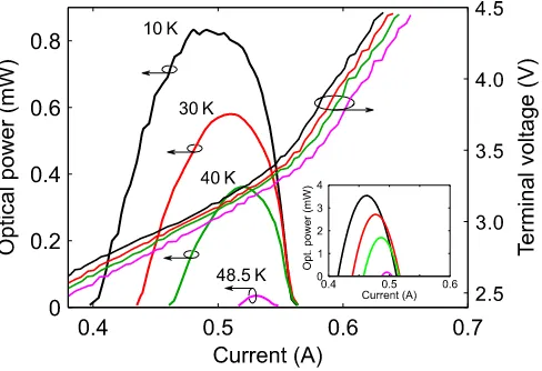
This approach properly reproduces the experimentally-measured light–current characteristics of the free-running QCL over its entire dynamic range of operation [39], when the collection efficiency of the detection system is accounted for. Figure 2 shows the laboratory measured light–current–voltage (L–I–V) characteristics of our exemplar QCL, for a range of cold finger temperatures. Inset in the figure, for comparison, are the calculated emitted optical power-current characteristics produced by the free-running model at the same temperatures. The calculated total emitted optical power is about four times higher than measured collected power at the detector due to limited collection efficiency of the detection equipment.

Fig. 2. Free-runningL–I–V characteristics of exemplar 2.59 THz BTC QCL. Main fig-ure: laboratory measured characteristic at four cold finger temperatures. Inset: Modeled characteristic at the same temperatures.

2.3. Incorporating Optical Feedback

Optical feedback is included in Eqs. (1) and (2) through the additional “feedback terms” identified by under braces. These equations (for photon density and phase, respectively) are derived from the Lang and Kobayashi model [13]. The feedback coupling coefficientκrelates to the emission facet mirror and target reflectivities (R2 and Rrespectively), and the re-injection loss ε as follows [17]:

κ=ε(1−R2) r

R R2

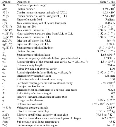
Table 1. Meaning of symbols used in Eqs. (1)–(5). Values for variables dependent on temperature and voltage are given at the instantt=1µs in the example below, at which timeT=46.1 K andV =2.94 V.

Symbol Description Value/Units

M Number of periods in QCL 90

S(t) Photon number 3.69×107

N3(t) Carrier number in upper lasing level (ULL) 1.03×107

N2(t) Carrier number in lower lasing level (LLL) 2.54×106

ϕ(t) Phase of electric field Radians

I(t) Total current into/out of device terminals 0.465 A

G(T,V) Gain factor [29] 1.42×104s−1

τ3(T,V) Total carrier lifetime in ULL 7.94 ×10−12s

τ32(T,V) Non-radiative relaxation time from ULL to LLL 1.52 ×10−10s

τ21(T,V) Total carrier lifetime in LLL 1.94 ×10−11s

η3(T,V) Injection efficiency into ULL 46.4 %

η2(T,V) Injection efficiency into LLL 0.60 %

τsp(T,V) Spontaneous emission lifetime 5.10×10−6s

τp Photon lifetime 9.02×10−12s

βsp Spontaneous emission factor 1.63×10−4

ωth Emission frequency at threshold (no optical feedback) 2.59 THz

τext Round-trip time of the external laser cavityτext=2Lextnext/c 11.3×10−9s

Lext External cavity length 1.704 m

next Refractive index of external cavity 1.00

τin Round-trip delay in laser diodeτin=2Linnin/c 3.92 ×10−11s

Lin Internal cavity length of laser 1.78 mm

nin Refractive index of internal laser cavity 3.30

κ Feedback coupling coefficient in external cavity 9.96×10−3

ε Re-injection loss factor 0.01

R2 Internal reflection coefficient of emitting laser facet 0.324

R Reflectivity of external target 0.7

α Henry’s linewidth enhancement factor [55] −0.1

q Charge on the electron 1.60×10−19C

k Boltzmann’s constant 8.62×10−5eV K−1

V(T,I) Voltage at device terminals 2.94 V

m Effective mass of laser chip 1.53×10−8kg

cp(T) Effective specific heat capacity of laser chip 79.6 J kg−1K−1 Rth(T) Effective thermal resistance — laser chip to cold finger 6.2 K W−1

T0(t) Sub mount/cold finger temperature 45 K

Values for the parameters in Eq. (6) are given in Table 1. The optical feedback path shown schematically in Fig. 3 is characterized byR,ε, and the external cavity round-trip timeτext= 2Lextnext/c, wherenextis the refractive index of the external cavity andcis the speed of light. In interferometric applications, any of these parameters may be manipulated to suit the requirements of the measurement being made. For example, variation ofLext(t) with time may represent a moving target or changes in surface relief during a raster scan over the object surface [16]; time variation ofε(t) orR(t) may represent an optical chopper in the collimated beam path; and the target reflectivity Rmay be a complex number for the purpose of a refractive index measurement [18]. The linewidth enhancement factor of THz QCLs,αin (2), is low and known to vary slightly with drive current and optical feedback [56]. In this work we use the value α=−0.1 [9].

Current pulser

Cold finger

QCL Emission

Back Injection Targe

t

M1 M2 M3

Thermal resistance

Temperature Controller

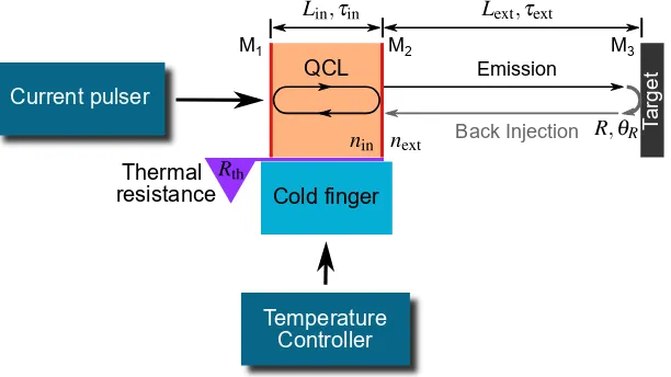
Fig. 3. Three-mirror optical feedback model. The internal cavity is the QCL active region with lengthLin, refractive indexnin, and round-trip propagation timeτin. Light leaves the internal cavity through the partially transmissive mirror M2, traverses the external cavity of lengthLextand refractive indexnextand is reflected back toward the QCL at target M₃. The proportion of light reflected by the target is the reflectivityRof M3and the phase change introduced by M₃isθ_R. The round-trip propagation time in the external cavity isτext. A portion of the reflected light, dictated by the re-injection lossε, re-enters the laser through M2and mixes with the field inside the laser cavity, altering the operating state of the laser.

2.4. Thermal model

Self-heating in QCLs is a significant contributor to temperature changes in the AR, with increases of> 10 K possible during long pulses [57]. Furthermore, the temperature-dependent RRE parametersτ31,τ32,τ21,η3,η2, andGcan change substantially over just a few kelvin. Thus, inclusion of a thermal model is vital in order to correctly predict QCL behavior when the AR temperature is changing. In addition, emission frequency (not modeled by our RREs) is markedly affected by temperature.

As the solution of the equation set progresses, each new temperature value obtained from (5) is fed back into the temperature-dependent parameters of the remaining equations, giving a self-consistent result. Even where the lattice temperature is not of direct interest, the thermal model must be solved in order to determine the constantly changing temperature-dependent RRE parameters in Eqs. (1)–(4).

The coefficientscp(T) andRth(T) in (5) are both strongly temperature dependent, especially at low operating temperatures (around 10 K) [58], making the coupled Eq. (5) highly non-linear. The specific heat capacitycp(T) for GaAs and AlGaAs increases non-linearly with temperature according to the Debye equation [59], and a third-order polynomial fit to measured data [60] was obtained for use in (5). The thermal resistanceRthof QCL ARs is both temperature-dependent and anisotropic, and can be up to ten times higher perpendicular to the quantum wells than in-plane [61, 62], owing to the enhanced phonon scattering at heterointerfaces [63]. Experimental studies reporting the temperature dependence ofRthare scarce, and our approach was thus to scale the measured temperature dependence of bulk GaAs’s thermal resistivity [64] to match a single laboratory measurement of our QCL’s Rth (8.2 K W−1 at 60 K). We then applied a polynomial fit to the resulting data, finding that a simple linear fit was satisfactory for the temperature range 10 K – 60 K.

For our QCL,cp(T) ranges from 1.0 to 114.0 J kg−1K−1andRth(T) from 0.7 to 8.2 K W−1over the temperature range 10 K – 60 K. Thus the notion of a “thermal time constant”τT=mcpRthis not particularly meaningful but, as will be seen, can be useful in describing AR thermal behavior at a specific temperature. The variability of bothcpandRthgive a very wide-ranging value ofτT, and hence within a single excitation pulse, thermal effects may be observable all the way from the timescale external of cavity dynamics to tens of microseconds [57].

2.5. Emission Frequency Modeling

As evident from Eqs. (1)–(4), the behavior of a laser under optical feedback depends strongly on the emission frequency, principally through the round-trip phase of the external cavity. The emission frequency of a QCL depends on the cold finger temperature and the laser driving current. The mechanisms responsible for the change in emission frequency with laser current are thermal and adiabatic in nature (i.e. caused by the changes in AR temperature and carrier density) [65,66]. Although the adiabatic mechanism is complex and non-linear, the linear component dominates in our QCL and provides a satisfactory approximation. For our exemplar modeling demonstration we used a laboratory-determined emission frequency coefficient of−12 MHz/mA for the driving current range of interest, 420 mA – 510 mA. Thermal frequency modulation is due to thermal expansion of the cavity [67] as well as change in refractive index with AR temperature [34]. The two effects together can produce a complex emission frequency vs. temperature characteristic which varies from laser to laser.

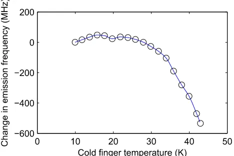
Figure 4 shows the measured emission frequency change vs. cold finger temperature for our exemplar BTC THz QCL. We use this data as the source for a behavioral model of emission frequency running concurrently with the RRE solver. We do this by mapping lattice temperature to cold finger temperature, and then interpolating with cubic splines to calculate the emission frequency used in the solver. This approach allows us to easily reproduce the relatively complex, non-linear temperature-dependent behavior of emission frequency while solving the RREs.

Emission frequency change due to the adiabatic and thermal mechanisms takes effect in our model by adjusting the value ofωth, the laser mode frequency in the absence of optical feedback at threshold, in Eqs. (1) and (2).

3. Results and Discussion

Fig. 4. Laboratory measured change in emission frequency with cold finger temperature, under static (cw) conditions. This characteristic is a result of change in both cavity length and refractive index change with temperature. Circles are the actual data points, with the curve to guide the eye.

conditions [13]. For laboratory work on THz QCLs, fast photo-detectors are presently bulky or expensive devices and the usual method is terminal voltage measurement. Our preference however is to present optical power output since it is a product of the model. Having calculated the temperature- and bias-dependent RRE parameters (a once-offoperation), Eqs. (1)–(5) may be repeatedly solved with a delay differential equation (DDE) solver for differing experimental conditions. The choice of experimental conditions includes selection of the external cavity lengthLext, target reflectivityR, cold finger temperatureT0, re-injection lossε, and drive current waveformI(t).

3.1. Picosecond and nanosecond regime — laser dynamics, external cavity effects,

and thermal effects

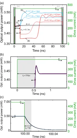
For this simulation we chose a 100 ns rectangular current pulse of amplitude 450 mA. This value of excitation current maximizes the thermal transient and optical output power for the purpose of illustration, while remaining within the region of positive slope efficiency. The cold finger temperature was set to 10 K and an external cavity lengthLext = 1.704 m was used, giving a round-trip time of 11.3 ns. We ran the simulation for target reflectivities of 0.0 (for reference), 0.3, and 0.7, and two slightly different external cavity lengths, the difference being 42.8µm — slightly less than a half-wavelength. This small distance change serves to illustrate the marked difference seen in the response with phase changes of aboutπ(or multiples thereof) in the external cavity. The values forα,τin,Lext,εgiven in Table 1, together withR =0.7, give a feedback coupling coefficientκ = 9.94×10−3 _{and Acket’s characteristic parameter} C = 2.90, placing the optical feedback in the moderate feedback regime [68]. ForR = 0.3 we have κ = 6.51 ×10−3 andC = 1.90. These conditions are typical of our experimental setup [18, 19] and are well-suited to illustrate the application of our model.

(red traces) — in this example, achieved by adding 42.8µm, about a half-wavelength, toLext. Changes inLextwill of course also alter the size of the settled self-mixing signal (compare solid blue and red traces after settling), where “self-mixing signal” is defined as the difference between outputs with and without optical feedback present.

In the first few nanoseconds the black trace (no feedback) can be seen to rise as a result of rapid temperature change at the start of the pulse, due to a small thermal time “constant”τT of around 16 ns. Thereafter, and near the end of the 100 ns pulse, the optical output settles as temperature changes more slowly. The temperature nevertheless continues to increase well into the microsecond regime, giving rise to relatively long-lasting effects. These are illustrated in the section to follow. The example of this section was chosen to illustrate thermal behavior observable in the nanosecond regime by usingT0=10 K. For higherT0, we have found that such effects are not be visible in this regime due to the longer thermal time constant associated with a higher AR temperature.

Picosecond scale effects, due purely to high-speed laser dynamics at turn on (in the absence of optical feedback), are shown in parts (b) and (c). In (b), we see the well-documented QCL overshoot without relaxation oscillation [69], and at turn-off(c), light remaining in the internal cavity decays with the expected photon lifetime. The four traces of part (a) are still present in (c) but not visible due to the much larger scale of the abscissa. Considering the narrow linewidths of THz QCLs (typically 1-2 meV, corresponding to about 1 ps [70]) and the nanosecond timescale of the shortest phenomena explored in this study, one could safely ignore the coherent interactions between the electronics and the electromagnetic field (photons).

3.2. Microsecond regime — thermal effects

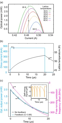
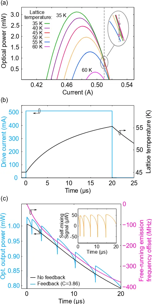
For the microsecond regime we chose a rectangular pulse of magnitude 465 mA and length 20µs, long enough to observe the effects associated with a thermal time constant of between 7µs (when T=45 K) and 12µs (when T∼55 K). The cold finger temperatureT0was set to 45 K, the external cavity length was 2.272 m, and target reflectivities of 0.0 (for reference) and 0.7 were used. ThisT0was chosen to obtain as large as possible a frequency change under pulsed operation, corresponding to the steep right-hand part of the emission frequency curve in Fig. 4. The results are shown in Fig. 6.

Part (a) shows the free-runningL–Icurves of the QCL at different lattice temperatures, with a vertical gray line tracing the operating point “trajectory” during the pulse. Dots denote the start and end conditions and an arrow head indicates chronological progression. Part (b) shows the response of lattice temperature to the drive pulse and part (c) the corresponding optical output power (blackR =0 “no feedback” trace and blue R=0.7 trace). In both cases, the decay in optical output is attributed to rising lattice temperature. The cause of the decay can be seen from part (a), which shows how light output falls with time and progressing lattice temperature while constant current is maintained during the pulse. The approximately exponential temperature trace in (b) (τT=7 to 12µs) thus maps via the trajectory to a similar (optical output) trace in (c). It should be noted that the staticL–Icurves in (a) for constantlatticetemperature are not the same as those inset in Fig. 2 (for constantcold fingertemperature).

Driv e curre nt (m A) 0 500 400 300 200 100 Lattice tem pera ture (K ) 55 50 45

0 5 10 15 20 25

Time (μs) (b)

0.42

Current (A)

0.46 0.50 0.54

(a) Optical pow er (m W) 3.0 2.5 2.0 1.5 1.0 0.5 Lattice temperature: 40 K 45 K 50 K 35 K 55 K 60 K (c) No feedback Feedback (C=3.86)

Opt. output powe

r (m

W)

0 10 20

Time (μs)

50 0 -50 Self-m ix ing Signa l ( μ W)

0 10 20 Time (μs)

−300 −200 −100 0 Free-runn ing em ission frequen cy of fset (MHz) −400 0.80 0.85 0.90 0.95 1.00 60 K 35 K

(c), which shows change in emission frequency during the driving pulse, is directly responsible for the self-mixing fringes when optical feedback is present, and is calculated by mapping lattice temperature in (b) using the frequency curve of Fig. 4.

To show the effect of pulse amplitude on the microsecond-scale response, we include a result for a 510 mA pulse magnitude in Fig. 7. Operating a QCL on the descending part of theL–I

curve is not usually performed in practice due to the negative effects of increased thermal loading, which include reduced bandwidth. However, in this case, it causes the trajectory to coincide with an operating regime in which a small change in output power with respect to the temperature is observed [see Fig. 7(a)], giving far less decay in optical output over the timescale of the driving pulse [blue curve in Fig. 7(c)]. Correspondingly, the self-mixing fringes in this case represent a relatively larger modulation depth of the output power. This would make it easier to filter out the self-mixing signal. Interestingly, there is a slight increase in the size of successive self-mixing peaks that is not present in the previous example — compare inset with that in Fig. 6(c).

4. Conclusion

We have presented a detailed model of a BTC THz QCL under optical feedback and pulsed operation, which allows prediction and exploration of lasing dynamics in not only applications relying on feedback, such as interferometry, but also applications in which feedback is incidental, such as free space communication. We reproduce observable phenomena such as bandwidth change, fringes due to adiabatic and thermal modulation, and chaotic behavior, and explore or discern the boundaries between the five operating regimes of the laser. These findings are of primary interest in developing new higher temperature optical feedback interferometry applica-tions with pulse-driven THz QCLs, and we propose that our modeling method will be useful in applications using other types of laser. For use with another laser the model would have to be adapted as required, depending on the type of laser. RREs and RRE parameters specific to the laser type, along with an appropriate thermal model, would then produce results representative of that laser type.

Funding