The impact of external disturbances on the performance of a cellular manufacturing systems

(1)

The impact of external disturbances on the performance of

a cellular manufacturing systems

SAAD, Sameh <http://orcid.org/0000-0002-9019-9636>

Available from Sheffield Hallam University Research Archive (SHURA) at:

http://shura.shu.ac.uk/14011/

This document is the author deposited version. You are advised to consult the

publisher's version if you wish to cite from it.

Published version

SAAD, Sameh (2016). The impact of external disturbances on the performance of a

cellular manufacturing systems. International Journal of Service and Computing

Oriented Manufacturing., 2 (1), 1-32.

Copyright and re-use policy

See

http://shura.shu.ac.uk/information.html

(2)

THE IMPACT OF EXTERNAL DISTURBANCES ON THE PERFORMANCE OF A CELLULAR MANUFACTURING SYSTEM

Sameh M Saad

Faculty of Arts, Computing, Engineering and Sciences, Department of Engineering and Mathematics

Sheffield Hallam University Sheffield, S1 2NU, UK e-mail: s.saad@shu.ac.uk

Biographical note: Sameh M. Saad is a Professor of Enterprise Modelling and Management, Postgraduate Research Coordinator and MSc/MBA Course Leader, in the Department of Engineering and Mathematics, Faculty of Arts, Computing, Engineering and Sciences, Sheffield Hallam University, UK. His research interests and experience include modelling and simulation, design and analysis of manufacturing systems, production planning and control, fuzzy AHP, logistics planning and control, reconfigurable manufacturing systems and next generation of manufacturing systems including fractal and biological manufacturing systems. He has published over 130 articles in various national and international academic journals and conferences, including keynote addresses and a book.

ABSTRACT

In manufacturing systems, different types of disturbances influence system’s performance, cellular

manufacturing has been proposed as an approach to cope with the uncertainty characteristic of customer driven markets. However, even cellular manufacturing systems are prone to the effects of varying demand patterns. In this study, the effects of some aspects related to demand variation such as the arrival of material, the variety of products and the variation in product mix are investigated to identify those system characteristics that -within the context of cellular manufacturing systems- represent an advantage in the presence of such disturbances. To do so, discrete event simulation is used to conduct the experimentation by modelling a cellular manufacturing system. Additionally, statistical design of experiment is employed to identify the factors contributing to higher system performance. The results show that, in spite of the demand related disturbance, machines with low set-up duration and highly skilled operators constitute the most important characteristics of an efficient manufacturing cell.

Keywords: cellular manufacturing system, manufacturing disturbances, simulation

1. INTRODUCTION

In a competitive environment characterized by a strong focus on satisfying each of the constantly

changing customers’ needs manufacturing systems are obliged to efficiently perform under a number of

(3)

Customer driven markets have an important influence on the arrivals of materials into the manufacturing

system. On the one hand, periods of low demand lead to a low utilization of the system’s resources; on the

other hand, periods of high demand lead to an increase in the arrival rate. Even though an increase in the arrival rate is associated with an increase in throughput and therefore an increase in income, similarly, an increase in the arrival rate inevitably leads to an increase in costly work-in-process (WIP) inventory. The

arrival of materials and its influence on system’s performance has been approached by a number of authors,

among those Tielemans and Kuik (1996) studied the relationship between batching of arrived orders and WIP

in order to reduce lead time; they recognised the impact long waiting times could have on system’s

performance. Chikamura et al. (1998) tested the influence of several lot arrival distributions on 7 production dispatching rules. The authors noticed that under most of the arrival scenarios, the best results were observed by a dispatching rule considering variables such as set-ups, waiting times and processing times. Govil et al. (1999) focused on the time of new lot arrivals in order to determine ways to predict average queue length at manufacturing resources. Prabhu (2000) claimed that arrival time determines the evolution of events in the manufacturing system, the sequence in which parts are processed and the machine idle time between processing parts. Given the important impact of arrival time on system’s performance, this author proposed the arrival time to be selected as a control variable in manufacturing systems. Moreover, Van Ooijen and Bertrand (2003) investigated the effects varying arrival rates have on throughput and WIP for a job shop; they concluded that an acceptable throughput would not necessarily imply a high arrival rate. In addition, they identified a trade-off between the costs associated with controlling the arrival rate and the revenues obtained by throughput.

Another implication of customer driven markets is an increasing demand for more variety. A higher product choice leads to more problems occurring in manufacturing systems; this is due to the level of complexity increasing along with variety. Research on product variety is a divergent topic; some views claim a significant impact of product variety on manufacturing performance, whereas other views suggest that there is actually no impact. MacDuffie et al. (1996) identified a trade-off associated to product variety; the authors noticed that whereas there is a higher revenue resulting from a wider variety, there are related higher costs and a loss of economies of scale as well. Although Fisher and Ittner (1999) acknowledged some common negative effects of variety, they also recognised that variety leads to benefits such as increased revenue. Berry and Cooper (1999) claimed that, in order to gain competitive advantage through product variety, it is necessary a proper alignment between marketing and manufacturing strategies in terms of process and infrastructure along with pricing and inventory. Randall and Ulrich (2001) argued that variety does not necessarily mean higher performance; they stated that regardless of variety strategies, the proper alignment between the supply chain and the product variety strategy is what is important. Thonemann and Bradley (2002) investigated the effects of product variety on supply chain performance and found that variety has an important effect on costs, especially when set-ups are significant. Fujimoto et al. (2003) stated that more variety causes less efficiency and higher costs; they presented a methodology to manage variety by synthesizing product-based and process-based approaches. Zhang et al. (2007) evaluated the impact of

response time and product variety strategies on system’s performance; they concluded that a higher

performance is achieved when both strategies are combined.

(4)

Liang et. al. (2011) studied the combination of virtual cells idea to construct new manufacturing systems in response to changing market dynamics. Egilmez et. al (2012) developed a non-linear mathematical model to the stochastic cellular manufacturing systems design problem to cope with a particular risk level, then simulated the obtained results to validate the proposed model and assess the performance of the designed cellular manufacturing system

The purpose of this study was to identify those components in a cellular manufacturing system contributing to maintain a higher system performance under the influence of external disturbances such as demand variations in both volume and pattern. This has been achieved by using the combined advantages of discrete event simulation and statistical design of experiments. The former was used to model a cellular manufacturing system with its main components; the latter provided the analysis structure for the identifications of those components with a major significance in terms of system performance. The consideration of both tools provided the capacity to adopt a wider perspective in the analysis and, therefore, not only did it facilitate the study of particular system components but also facilitated the study of the interactions occurring within the system.

2. RESEARCH METHOD

2.1.Simulation model

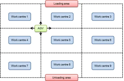
[image:4.595.94.505.377.648.2]

Discrete event simulation has been used to represent a semi-automated cellular manufacturing system consisting of 9 different work centres. Each work centre comprises one input buffer, one machine and one output buffer. All the work centres are connected by an automated material handling system. Each work centre is assisted by one of the six operators within the cell whose job basically consists on loading, controlling and unloading machines. Figure 1 graphically represents the cellular system previously described.

Figure 1: Cellular Manufacturing System Layout

2.2.Simulation model operation assumptions

The following are list of the assumptions considered during the development of the simulation model:

2.2.1.Parts

 Parts arrive in the system one at a time and following an exponential distribution with an average

(5)

 There are five different products involved; each product with different processing requirements, i.e. different processing times and routes. Process routing is fixed for each of the products.

2.2.2.Machines

 Each machine represents a specific manufacturing process within the system, therefore their different

operative features.

 Machines can process only one piece at a time.

 Although all of the machines are assumed to follow a normal distribution in both processing and set

up times, the times are different from each other.

 There is a different usage cost per minute associated to each machine.

 Machines do not have any automation level, therefore each machine do require an operator.

 It is assumed that all machines breakdown from time to time, consequently a different efficiency level

has been predefined for each machine.

 When machines fail, repairs are assumed to be done by external personnel (not considered for the

purposes of this research). Machine repairs are assumed to follow an exponential distribution with different average times for each machine.

2.2.3.Buffers

 Blocking does not occur.

 Buffer capacity is limited; all the buffers have the same capacity. There is a storage cost per item per

minute associated to the capacity, i.e. the higher the capacity the higher the storage cost.

 Parts in buffers are prioritized according to FIFO dispatching rule, i.e. parts are dispatched either into

a machine or vehicle considering a first come first served rule.

2.2.4.Operators

 Operators have different abilities; in consequence labour cost is associated to the skill level.

 Operators are assumed not to be always available, therefore different availability percentages and

absence times have been specified for each operator.

 Travelling times for operators have not been considered.

2.2.5.AGV

 The material handling system is totally independent from human operators.

 The AGV travels at a constant speed along a fixed route connecting all the work centres.

 Material handling costs are omitted and no vehicle breakdowns are assumed.

 The AGV’s travelling time is determined based on its speed.

2.2.6.Finished product

 Revenue per finished product regardless of its type has been assumed.

2.3.Model Verification

Model verification can be carried out in three different and complementary ways: Checking the code, performing visual checks, and inspecting output reports (Robinson, 1994). Code checking was facilitated by the capabilities of the simulation software, which made possible to interactively check the coding line by line. Visual checks were performed by keeping track of parts progressing throughout the system, allowing the behaviour of all the components intervening along the process to be monitored. Additionally, the model was run in an event-by-event mode in order to complement the verification process. This verification procedure made possible to guarantee that each element within the model would behave as it was originally intended. The last method of model verification consisted in checking the outputs of the main components within the model; to do so 30 replications, each with a run time of 400 simulation-hours, were conducted. After analysing some of the most important system outputs it was possible to confirm that all the model components performed according to what had been defined during the model coding process.

2.4.Model validation

(6)

judged upon the viability of making decisions based on the information provided by the simulation model. Ideally, a model would be better validated when compared to a real system (Pidd, 1993); however, models do not always represent real systems. Because the latter is the case in the present research, it was not necessary to compare the model with either empirical data or the behaviour of a real system (Maki and Thompson, 2006). Validation techniques are classified in two groups, namely subjective techniques and objective techniques. Objective validation-techniques do require the existence of real systems in order to establish input-output comparisons between systems. Subjective techniques, as their name imply, does not necessarily require the

existence of a real system since they are more dependent on the experience and “feelings” of its developers

(Banks, 1998). The proposed model has been validated using a sensitivity analysis as a subjective validation method. The sensitivity analysis capability is a built-in feature in Simul8; its function is to test the assumed probability distributions in terms of how sensitive the results are to changes in these inputs. A number of probability distributions particularly related to machine processing times and set-ups have been randomly selected to be tested. The sensitivity analysis confirmed the validity of the assumptions.

2.5.Experimental design

A minimum model warm-up period of 50 hours was calculated by using Welch’s graphical method. A minimum run length of 220 hours was also calculated by a graphical approach. Both approaches are described

in Robinson’s (1994).

To measure the performance of the modelled manufacturing cell three different response variables were selected, namely number of completed parts, total cost and average time in the system. Regarding the design factors, three aspects related to work centres and three aspects related to the material handling sub-system were selected, those are the following:

1. The skill level of operators. It is determined by the number of different machines a single operator is able to control.

2. The capacity of inter-storage buffers. It is related to the maximum number of parts the system is able to hold.

3. The duration of machine set-ups. It is the time it takes for machines to switch from producing one specific type of part to producing a completely different type of part.

4. The number of AGVs. It is related to the total number of material handling vehicles within the system. 5. The speed of AGVs. It is the distance covered by material handling vehicles during a specific period

of time.

6. The loading capacity of AGVs. The maximum number of parts a material handling vehicle can transport between work centres.

To investigate the effects of external disturbances on the performance of the modelled manufacturing cell, four different scenarios were considered as shown in the following subsections.

2.5.1.Irregular pattern of raw material arrivals

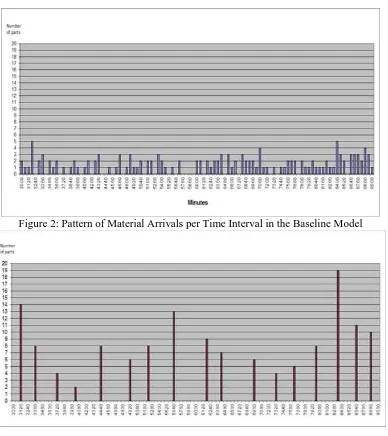
This scenario simulates the situation in which, due to some external cause such as demand variation or supply delays, the pattern of raw-material-arrivals into the system is disrupted in such a way that there is a higher variation in both the time between arrivals and the arriving number of parts. The variation in the arrival pattern in this scenario with respect to the arrival pattern in the baseline model is contrasted in figures 2 and 3 below.

In order to generate the pattern of arrivals in figure 3 a gamma distribution has been used. The parameters

used in the gamma distribution generating the interarrival times in this scenario are a shape parameter (α) of

10 minutes and a scale parameter (β) of 38 minutes. Additionally, a normal distribution with an average of 10

(7)

[image:7.595.107.495.64.500.2]

Figure 2: Pattern of Material Arrivals per Time Interval in the Baseline Model

Figure 3: Pattern of Material Arrivals per Time Interval in the Disturbance Scenario

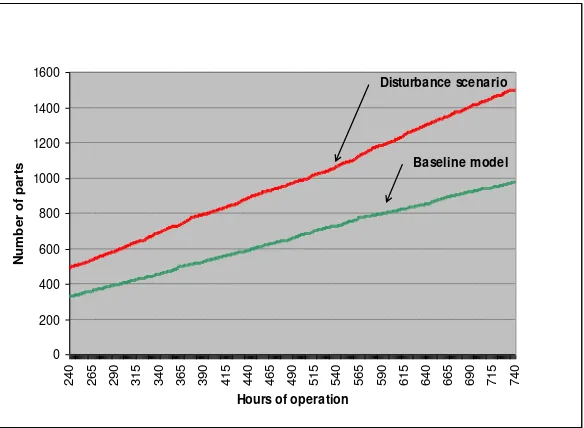
2.5.2.Increased arrivals of raw material scenario

As opposed to the previous scenario, in this scenario the pattern of material arrivals is not modified but amplified in order to simulate a condition where the MS needs to cope with an unexpected increase in production orders. Figure 4 shows the difference between arrivals of raw material in the baseline model and arrivals of material in the disturbance scenario.

(8)

[image:8.595.147.439.85.299.2]

Figure 4: Number of Raw Materials Arrivals

2.5.3.Increased product variety scenario

[image:8.595.207.389.430.611.2]

The range of parts produced by the system has been increased from 5 to 10 parts in this scenario; each part has different processing characteristics. Since the purpose is to investigate product variety and not product mix variation, the product mix range in this scenario with respect to the baseline model has been increased by only 2%. Table 1 compares the increased product variety in this scenario with respect to the product variety in the baseline model.

Table 1: Comparison of Product Varieties

Product Baseline model

Disturbanc e scenario

1 23% 10%

2 17% 9%

3 20% 7%

4 18% 8%

5 22% 6%

6 N/A 13%

7 N/A 14%

8 N/A 11%

9 N/A 12%

10 N/A 10%

TOTAL 100% 100%

2.5.4.High variation in product mix scenario

[image:8.595.200.398.710.760.2]

As opposed to the previous scenario where a wider choice of products is investigated, this scenario explores the demand variation existing among products. To simulate this scenario, the same five original products defined in the baseline model are considered, however, the product mix has been adjusted in order to reflect a bigger difference in the demand for each product in relation to the rest of the products. Table 2 illustrates a comparison between the original product mix and the mix considered in this scenario.

Table 2: Comparison of Product Mix Product Baseline Disturbance

1 23% 18%

2 17% 3%

0 200 400 600 800 1000 1200 1400 1600

240 265 290 315 340 365 390 415 440 465 490 515 540 565 590 615 640 665 690 715 740

Hours of operation

N

um

be

r

of

pa

rt

s Baseline model

(9)

3 20% 26%

4 18% 8%

5 22% 45%

total 100% 100%

Range 6% 42%

It can be noticed from the table 2 above that the range in the product mix for the disturbance scenario is considerably larger than the range in the baseline model.

3. MODEL REPLICATIONS AND DATA ANALYSIS

The number of necessary replications for each simulation scenario was determined by calculating a maximum error estimate out of a series of initial model replications. The maximum error estimate together with a desired error was taken into account to determine the required number of replications for each model. According to such calculation, a minimum of 250 replications per model were enough to guarantee statistical reliability.

Considering that there were 6 design factors involved, each at two levels, a 26 full factorial design was employed. Given the high variation in the resulting data related to the responses cost and time, the original data has been normalized using a log transformation. Subsequently an analysis of variance was conducted to identify the significant factors. Main effects plots and interaction plots were used to identify factor levels and factor interactions respectively. Minitab was the statistical software used to analyse the data generated by each simulation scenario.

4. RESULTS

The following sections report on the obtained results including the analysis of variance.

4.1. Irregular pattern of raw material arrivals

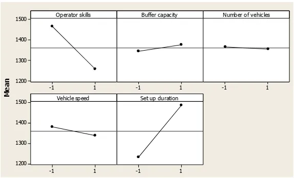
After conducting an analysis of variance and calculating the factor effect estimates for each of the considered responses, the most important effects were confirmed by the main effects plots in figures 5, 6 and 7.

In terms of the number of completed parts, figure 5 and the factor effect estimates in appendix 1 indicated that four influential factors are: high operator skills, high buffer capacity, high number of vehicles and low duration of machine set-ups; all with a combined percent contribution of approximately 61%. Although high vehicle speed also appeared as main effect in figure 5, its percent contribution was only of 1%.

In figure 6 two key factors to minimize cost were identified, namely low buffer capacity and low duration of machine set-ups; both with a combined percent contribution of 96%. Although low operator skills and low number of vehicles also appeared in figure 6 as main effects, the calculation of effect estimates in appendix 1 indicated a low percent contribution of 1.5%.

(10)

[image:10.595.144.452.70.262.2] [image:10.595.144.453.323.512.2]

Figure 4: Main Effect Plot for Parts

Figure 5: Main Effect Plot for Cost

Figure 6: Main Effect Plot for Time

1 -1 786 784 782 1

-1 -1 1

1 -1 786 784 782 1 -1 Operator skills M e a n

Buffer capacity Number of v ehicles

Vehicle speed Set up duration

Data Means 1 -1 65000 60000 55000 50000 45000 1 -1 1 -1 65000 60000 55000 50000 45000 1 -1 Operator skills M e a n Buffer capacity

Number of vehicles Set up duration Data Means 1 -1 1500 1400 1300 1200 1

-1 -1 1

1 -1 1500 1400 1300 1200 1 -1

Operator sk ills

M

e

a

n

[image:10.595.154.441.547.721.2]

(11)

[image:11.595.154.444.69.259.2]

4.2. Increased arrivals of raw material

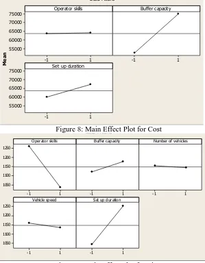
The main effect plots in figures 8, 9 and 10 validated the significant factors previously identified by the analysis of variance.

As shown by figure 8, to achieve a maximum number of completed parts, high operator skills, high buffer capacity and low duration machine set-ups were the most significant factors with a combined percent contribution of approximately 67%.

[image:11.595.149.448.365.749.2]

1 -1 1000 999 998 997 996 1 -1 1 -1 1000 999 998 997 996 Operator skills M e a n Buffer capacity

Set up duration

Data Means 1 -1 75000 70000 65000 60000 55000 1 -1 1 -1 75000 70000 65000 60000 55000 Operator skills M e a n Buffer capacity

Set up duration

Data Means 1 -1 1250 1200 1150 1100 1050 1

-1 -1 1

1 -1 1250 1200 1150 1100 1050 1 -1

O perator sk ills

M

e

a

n

(12)

As shown in figure 8, to achieve a maximum number of completed parts, high operator skills, high buffer capacity and low duration machine set-ups were the most significant factors with a combined percent contribution of approximately 67% according to appendix 2.

Figure 9 confirms that low buffer capacity and low duration of machine set-ups, both with a combined percent contribution of approximately 97% according to appendix 2, were the most significant factors to achieve minimum cost.

[image:12.595.148.469.224.428.2]

Concerning a minimum time in the system, figure 10 shows that high operator skills, low duration of machine-set ups and low buffer capacity are the three most influential factors with a combined percent contribution of approximately 88% consistent with appendix 2. A high number of vehicles and high vehicle speed, both with a combined percent contribution of nearly 1%, were not influential enough.

4.3. Increased product variety

After conducting an analysis of variance the most significant factors in a scenario characterised by a wider product variety have been confirmed by figures 11, 12 and 13.

Figure 11: Main Effect Plot for Cost 1

-1 667.0

666.5

666.0

665.5

1 -1

667.0

666.5

666.0

665.5

1 -1

Operator skills

M

e

a

n

Buffer capacity

Number of vehicles Set up duration Data Means

1 -1

65000

60000

55000

50000

45000

1 -1

65000

60000

55000

50000

45000

Operator skills

M

e

a

n

Buffer capacity

Set up duration

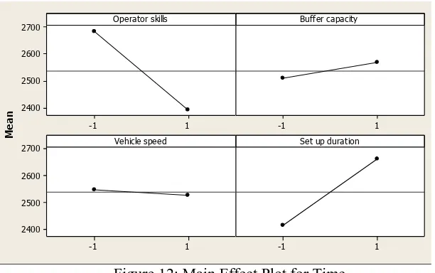
[image:12.595.146.450.530.717.2]

(13)

[image:13.595.146.452.71.263.2]

Figure 11 indicates that, to achieve a maximum number of completed parts, the first and most significant factor was high operator skills with a percent contribution of 26%, followed by high buffer capacity with a percent contribution of 23%; the third and fourth important factors were low duration of machine set-ups and high number of vehicles with percent contributions of 6% and 5.6% respectively.

Figure 12 shows that there were only two main factors for achieving minimum cost, those were low buffer capacity and low duration of machine set-ups, both with a combined percent contribution of approximately 97%.

[image:13.595.182.433.420.566.2]

Figure 13 confirmed that, to minimize time in the system, high operator skills and low duration of machine set-ups were key factors with a combined percent contribution of approximately 87% (see appendix 3 for the percent contributions of each factor in terms of the three considered response variables).

Figure 13: Main Effect Plot for Parts 4.4 High variation in product mix

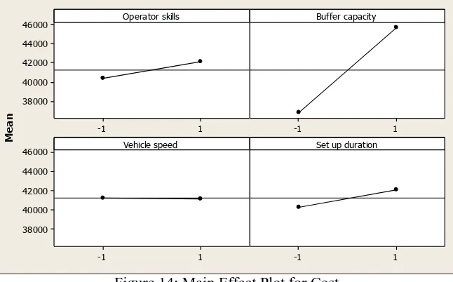
Figures 14, 15 and 16 show the most influential factors in achieving higher performance in a scenario characterized by high variation in product mix. See appendix 4 for the analysis of variance from where the initial significant factors were identified.

Figure 14 shows that, in terms of a maximum number of completed parts, the only two significant factors were high duration of machine set-ups and low operator skills, both with a combined percent contribution of approximately 24%. The analysis of variance in appendix 4 shows that an important interacting factor to achieve a higher number of parts was high vehicle speed.

Figure 15 confirms that, in terms of minimum cost, low buffer capacity was the most influential factor with a percent contribution of 92% according to appendix 4. Low operator skills and low duration of machine set-ups were also important factors with a significantly lower percent contribution of 4% each.

1 -1

2700

2600

2500

2400

1 -1

2700

2600

2500

2400

1 -1

Operator skills

M

e

a

n

Buffer capacity

Data Means

1 -1

668.3

668.2

668.1

668.0

667.9

1 -1

Operator skills

M

e

a

n

(14)

[image:14.595.136.459.72.273.2] [image:14.595.137.463.72.506.2]

Although figure 15 shows the existence of five significant factors in terms of minimum time in the system, according to appendix 4 only three factors were truly significant; those were high operator skills, low duration of machine set-ups and high vehicle speed; all with a combined percent contribution of approximately 92%.

5. DISCUSSION AND FUTURE WORK

As it was mentioned at the beginning of this study, demand aspects such as volume and pattern are among

some of the factors affecting manufacturing cell’s performance. As Van Ooijen and Bertrand (2003) claimed,

periods of high and low demand lead to unbalanced workload and variation in resource utilization. The same authors identified the trade-off existing between a higher throughput resulting from an increase in the arrival rate and higher costs particularly associated to high levels of WIP inventory. In addition to approaches like arrival rate control policies, other mechanisms to cope with material arrivals associated problems have been identified in this study. To achieve a maximum number of completed parts in scenarios characterized by either irregular or increased arrivals of raw material, the most important factors identified in this study were highly skilled operators and high buffer capacity. These same factors also were the most influential to achieve a maximum number of parts in a scenario characterized by increased product variety. Highly skilled operators are important especially during periods of high demand in order to guarantee better resource utilization. A higher buffer capacity is similarly necessary to store the excess of WIP inventory originated during those periods. In scenarios characterized by a high variation in product mix, dedicated operators are more suitable

1 -1

46000

44000

42000

40000

38000

1 -1

46000

44000

42000

40000

38000

1 -1

Operator skills

M

e

a

n

Buffer capacity

Data Means

1 -1

1450

1400

1350

1300

1

-1 -1 1

1 -1

1450

1400

1350

1300

1 -1

Operator sk ills

M

e

a

n

(15)

since old products, going through the last stage of their life cycle, will experience a low demand allowing more resource attention to be paid on products with higher demand.

The trade-off existing between the responses throughput and high costs resulting from high levels of WIP inventory, has been mentioned in the previous paragraph. The experiments conducted in this study have shown that, in all of the considered disturbance scenarios, the two most important factors were low buffer capacity and low duration of machine set-ups. High costs resulting from high WIP inventory levels can be overcome by limiting WIP levels; this can be achieved by setting work centres with low buffer capacity. Scenarios of variation in the demand pattern like product variety and product mix are particularly associated to higher costs. On the one hand, a product variety scenario implies higher costs associated to lower economies of scale, more set-ups and lower labour productivity (Thonemann and Bradley, 2002). On the other hand, a product mix scenario involves increased manufacturing costs resulting from increased heterogeneity in process specifications of a product mix (Anderson, 1995). Therefore low duration of machine set-ups is another characteristic that needs to be considered to reduce costly WIP inventories, particularly those caused by variation in the demand pattern.

To cope with a changing environment, a crucial task to a quicker throughput and to an improved performance is lead time reduction. In order to achieve a reduced job flow time, improvements in delivery speed have been proposed along with improvements in WIP inventory and response to market requirements (Deane and Yang, 1992). In the manufacturing system analysed in the present study, two essential features to achieve the minimum time in the system were highly skilled operators and low duration of machine set-ups. These two characteristics were the most significant ones for all of the considered scenarios. Similarly, high speed of vehicles was other factor that resulted significant exclusively for the scenario involving high variation in product mix.

Looking at the whole picture, the system’s features that consistently resulted significant for all the considered scenarios, in terms of the three considered performance measures, were low set-ups duration in the first place followed by highly skilled operators. Cellular manufacturing systems with similar operating characteristics to those specified in this study, and which are constantly facing frequent changes in the volume and pattern of the demand, may find that, counting on versatile machines able to accomplish quick changeovers and skilled human operators able to keep the system operating under different circumstances, are key characteristics to maintain an acceptable performance.

Future work on the topic could adopt a wider perspective on the origin of disturbances affecting manufacturing systems. Both internal and external disturbances could be considered to investigate their effect on performance and to identify aspects providing manufacturing systems the capability to cope with a number of disrupting situations. To complement the present study, it would be interesting to consider a range of variation in the intensity of disturbances and identify how certain system characteristics become significant at varying disturbance intensities. Moreover, other systems layouts could be investigated to confirm the advantages offered by cellular manufacturing against uncertainty. Another important aspect to consider in future research is related to the implications for the manufacturing system to hold a certain degree of flexibility, i.e. the effects, in terms of different performance measures, of system adjusting to a number of situations, together with the trade-offs involved.

REFERENCES

Anderson, S. W., 1995. Measuring the impact of product mix heterogeneity on manufacturing overhead costs. Accounting Review, 70, 363-387.

Anderson, S. W., 2001. Direct and indirect effects of product mix characteristics on capacity management decisions and operating performance. The international journal of flexible manufacturing systems, 13, 241-265.

Banks, J., 1998. Handbook of Simulation: Principles, methodology, advances, applications, and practise. 1998, New York: John Wiley & Sons.

Berry, W. L. and Cooper, M. C., 1999. Manufacturing flexibility: methods for measuring the impact of product variety on performance in process industries. Journal of Operations Management, 17, 163-178. Chikamura, A., Nakamae, K. and Fujioka, H., 1998. Influence of lot arrival distribution on production

(16)

Deane, R. H. and Yang, J. Q., 1992. Product mix selection and closed manufacturing cell flow time performance. International Journal of Production Economics, 28, 157-169.

Egilmez, G., Suer, G.A. and Huang, J., 2012. Stochastic cellular manufacturing system design subject to maximum acceptable risk level, Computers & Industrial Engineering, 63, 842-854.

Fisher, M. L. and Ittner, C. D., 1999. The impact of product variety on automobile assembly operations: Empirical evidence and simulation analysis. Management Science, 45, 771-786.

Fujimoto, H., Ahmed, A., Iida, Y. and Hanai, M., 2003. Assembly process design for managing manufacturing complexities because of product varieties. International Journal of Flexible Manufacturing Systems, 15, 283-307.

Govil, M., Minis, I. and Proth, J., 1999. Prediction of average queue length in manufacturing resources at the time of new lot arrival. Applies Stochastic Models in Business and Industry, 15, 111-121.

Liang, F., Fung, R.Y.K. and Jiang, 2011. Modelling approach and behaviour analysis of manufacturing resources in virtual cellular manufacturing systems using resource element concept. International Journal of Computer Integrated Manufacturing, 24, 12, 1168-1182.

Macduffie, J. P., Sethuraman, K. and Fisher, M. L., 1996. Product variety and manufacturing performance: Evidence from the International Automotive Assembly Plant Study. Management Science, 42, 350-369. Maki, D. and M. Thompson, 2006. Mathematical Modeling and Computer Simulation, Belmont, Ca.:

Thomson Higher Education.

Pidd, M., 1993. Computer simulation in management science. 3rd. ed. 1993, Chichester: John Wiley & Sons. Prabhu, V., 2000. Performance of real-time distributed arrival time control in heterarchical manufacturing

systems. IEE Transactions 32, 323-331.

Randall, T. and Ulrich, K., 2001. Product variety, supply chain structure, and firm performance: Analysis of the US bicycle industry. Management Science, 47, 1588-1604.

Robinson, S., 1994. Successful Simulation: A Practical Approach to Simulation Projects, London, McGraw-Hill.

Seifoddini, H. and Djassemi, M., 1996. Sensitivity analysis in cellular manufacturing system in the case of product mix variation. Computers & Industrial Engineering, 31, 163-167.

Seifoddini, H. and Djassemi, M., 1997. Determination of a flexibility range for cellular manufacturing systems under product mix variations. International Journal of Production Research, 35, 3349-3366.

Thonemanu, U. W. and Bradley, J. R., 2002. The effect of product variety on supply-chain performance. European Journal of Operational Research, 143, 548-569.

Tielemans, P. and Kuil, R., 1996. An exploration of models that minimize lead time through batching of arrived orders. European Journal of Operational Research, 95, 374-389.

Van Ooijen, H. and Bertrand, J., 2003. The effects of a simple arrival rate control policy on throughput and work-in-process in production systems with workload dependent processing rates. International Journal of Production Economics, 85, 61-68.

(17)

Appendix 1

Irregular pattern of raw material arrivals

ANOVA table for number of completed parts

ANOVA table for cost

Source DF SS MS F P Operator skills 1 147.235 147.235 213.66 0.000* Buffer capacity 1 425.998 425.998 618.18 0.000* Number of vehicles 1 88.477 88.477 128.39 0.000* Vehicle speed 1 12.056 12.056 17.50 0.000* Set up duration 1 109.464 109.464 158.85 0.000* Operator skills*Buffer capacity 1 50.887 50.887 73.84 0.000* Operator skills*Number of vehicles 1 6.997 6.997 10.15 0.003* Operator skills*Vehicle speed 1 31.981 31.981 46.41 0.000* Operator skills*Set up duration 1 20.545 20.545 29.81 0.000* Buffer capacity*Number of vehicles 1 31.927 31.927 46.33 0.000* Buffer capacity*Vehicle speed 1 9.938 9.938 14.42 0.000* Buffer capacity*Set up duration 1 126.527 126.527 183.61 0.000* Number of vehicles*Vehicle speed 1 36.386 36.386 52.80 0.000* Number of vehicles*Set up duration 1 4.669 4.669 6.78 0.013 Operator skills*Buffer capacity* 1 35.869 35.869 52.05 0.000* Number of vehicles

Operator skills*Buffer capacity* 1 28.375 28.375 41.18 0.000* Vehicle speed

Operator skills*Buffer capacity* 1 37.340 37.340 54.19 0.000* Set up duration

Buffer capacity*Number of vehicles* 1 26.815 26.815 38.91 0.000* Vehicle speed

Operator skills*Number of vehicles* 1 4.137 4.137 6.00 0.019 Vehicle speed

Operator skills*Buffer capacity* 1 5.270 5.270 7.65 0.009* Number of vehicles*Vehicle speed

Operator skills*Number of vehicles* 1 0.540 0.540 0.78 0.381 Set up duration

Buffer capacity*Number of vehicles* 1 0.031 0.031 0.05 0.832 Set up duration

Operator skills*Buffer capacity* 1 9.529 9.529 13.83 0.001* Number of vehicles*Set up duration

Error 40 27.565 0.689 Total 63 1278.560

S = 0.830128 R-Sq = 97.84% R-Sq(adj) = 96.60%

Source DF SS MS F P Operator skills 1 0.007388 0.007388 521.53 0.000* Buffer capacity 1 0.441267 0.441267 31151.52 0.000* Number of vehicles 1 0.000091 0.000091 6.42 0.014 Vehicle speed 1 0.000001 0.000001 0.08 0.777 Set up duration 1 0.052641 0.052641 3716.25 0.000* Operator skills*Buffer capacity 1 0.008019 0.008019 566.11 0.000* Operator skills*Set up duration 1 0.000189 0.000189 13.35 0.001* Buffer capacity*Set up duration 1 0.000785 0.000785 55.45 0.000* Number of vehicles*Set up duration 1 0.000442 0.000442 31.20 0.000* Vehicle speed*Set up duration 1 0.000294 0.000294 20.74 0.000* Operator skills*Buffer capacity* 1 0.000609 0.000609 43.00 0.000* Set up duration

Error 52 0.000737 0.000014 Total 63 0.512463

(18)

Appendix 1 (continued)

ANOVA table for time in the system

Factor effect estimates for parts, cost and time

Source DF SS MS F P Operator skills 1 0.067812 0.067812 2535.35 0.000* Buffer capacity 1 0.001391 0.001391 52.00 0.000* Number of vehicles 1 0.000367 0.000367 13.72 0.001* Vehicle speed 1 0.003492 0.003492 130.56 0.000* Set up duration 1 0.102952 0.102952 3849.14 0.000* Operator skills*Buffer capacity 1 0.001749 0.001749 65.38 0.000* Operator skills*Number of vehicles 1 0.000848 0.000848 31.69 0.000* Operator skills*Vehicle speed 1 0.000455 0.000455 17.00 0.000* Operator skills*Set up duration 1 0.006727 0.006727 251.52 0.000* Number of vehicles*Vehicle speed 1 0.000674 0.000674 25.20 0.000* Number of vehicles*Set up duration 1 0.001361 0.001361 50.87 0.000* Vehicle speed*Set up duration 1 0.001310 0.001310 48.99 0.000* Number of vehicles*Vehicle speed* 1 0.000675 0.000675 25.23 0.000* Set up duration

Error 50 0.001337 0.000027 Total 63 0.191149

S = 0.00517172 R-Sq = 99.30% R-Sq(adj) = 99.12%

Number of completed

parts Cost Time in the system

Model term Percent contributi on Model term Percent contributi on Model term Percent contributi on Operators

skills 11.52%

Operators

skills 35.47% Buffer

capacity 33.32%

Buffer

capacity 86.11% Number of

vehicles 6.92% Set-up

duration 8.56%

Set-up

duration 10.27%

Set-up

duration 53.87% Rest of main

factors 1.01%

Rest of main

factors 1.46%

Rest of main

factors 2.75%

Buffer capacity x

set-up duration 9.89% Buffer capacity x set-up duration 0.15% Operators skills x Buffer capacity x set-up duration

2.92%

Operators skills x Buffer

capacity x set-up duration

0.12%

(19)

Rest of

interactions 23.01%

Rest of

interactions 1.89%

Rest of

interactions 4.39%

(20)

Appendix 2

Increased arrivals of raw material

Source DF SS MS F P Operator skills 1 218.423 218.423 154.05 0.000* Buffer capacity 1 68.337 68.337 48.20 0.000* Number of vehicles 1 3.301 3.301 2.33 0.133 Set up duration 1 17.520 17.520 12.36 0.001* Operator skills*Buffer capacity 1 20.117 20.117 14.19 0.000* Operator skills*Set up duration 1 28.457 28.457 20.07 0.000* Buffer capacity*Number of vehicles 1 19.280 19.280 13.60 0.001* Error 56 79.401 1.418

Total 63 454.834

S = 1.19075 R-Sq = 82.54% R-Sq(adj) = 80.36%

Source DF SS MS F P Operator skills 1 0.001188 0.001188 47.57 0.000* Buffer capacity 1 0.381058 0.381058 15254.05 0.000* Set up duration 1 0.037660 0.037660 1507.56 0.000* Operator skills*Buffer capacity 1 0.010078 0.010078 403.42 0.000* Operator skills*Set up duration 1 0.001401 0.001401 56.09 0.000* Buffer capacity*Set up duration 1 0.001014 0.001014 40.58 0.000* Operator skills*Buffer capacity* 1 0.000666 0.000666 26.66 0.000* Set up duration

Error 56 0.001399 0.000025 Total 63 0.434464

(21)

Source DF SS MS F P Operator skills 1 0.107060 0.107060 2446.42 0.000* Buffer capacity 1 0.005619 0.005619 128.41 0.000* Number of vehicles 1 0.000533 0.000533 12.18 0.001* Vehicle speed 1 0.001696 0.001696 38.75 0.000* Set up duration 1 0.093452 0.093452 2135.48 0.000* Operator skills*Buffer capacity 1 0.005592 0.005592 127.79 0.000* Operator skills*Number of vehicles 1 0.001251 0.001251 28.59 0.000* Operator skills*Set up duration 1 0.010382 0.010382 237.23 0.000* Number of vehicles*Vehicle speed 1 0.000454 0.000454 10.37 0.002* Number of vehicles*Set up duration 1 0.002151 0.002151 49.15 0.000* Vehicle speed*Set up duration 1 0.000394 0.000394 9.00 0.004* Buffer capacity*Set up duration 1 0.000333 0.000333 7.62 0.008 Operator skills*Buffer capacity* 1 0.000500 0.000500 11.42 0.001* Set up duration

Error 50 0.002188 0.000044 Total 63 0.231605

S = 0.00661527 R-Sq = 99.06% R-Sq(adj) = 98.81%

skills 48.02%

Operators

capacity 15.03% Buffer capacity 87.71% Set-up

duration 3.85%

Set-up

duration 8.67%

Set-up

factors 1.24%

Rest of main

factors 0.58%

Rest of main

factors 3.41% Operators

skills x set-up duration

6.26%

Operators skills x set-up

duration

4.48%

capacity

4.42%

capacity

2.32%

Rest of

interactions 21.18%

Rest of

interactions 0.72%

Rest of

interactions 5.53%

(22)

Appendix 3

Increased product variety

Source DF SS MS F P Operator skills 1 41.9398 41.9398 98.59 0.000* Buffer capacity 1 37.2434 37.2434 87.55 0.000* Number of vehicles 1 8.9803 8.9803 21.11 0.000* Vehicle speed 1 0.6831 0.6831 1.61 0.213 Loading capacity 1 0.0241 0.0241 0.06 0.813 Set up duration 1 9.5636 9.5636 22.48 0.000* Operator skills*Buffer capacity 1 8.9670 8.9670 21.08 0.000* Operator skills*Number of vehicles 1 0.0088 0.0088 0.02 0.886 Operator skills*Vehicle speed 1 0.1441 0.1441 0.34 0.564 Operator skills*Loading capacity 1 0.0923 0.0923 0.22 0.644 Operator skills*Set up duration 1 11.9461 11.9461 28.08 0.000* Buffer capacity*Number of vehicles 1 3.9882 3.9882 9.38 0.004* Buffer capacity*Vehicle speed 1 0.0595 0.0595 0.14 0.710 Buffer capacity*Set up duration 1 0.0500 0.0500 0.12 0.733 Number of vehicles*Vehicle speed 1 0.0232 0.0232 0.05 0.817 Number of vehicles*Set up duration 1 0.0076 0.0076 0.02 0.894 Vehicle speed*Set up duration 1 0.6952 0.6952 1.63 0.209 Loading capacity*Set up duration 1 3.6001 3.6001 8.46 0.006* Operator skills*Buffer capacity* 1 1.9748 1.9748 4.64 0.037* Number of vehicles

Operator skills*Buffer capacity* 1 2.5394 2.5394 5.97 0.019* Vehicle speed

Operator skills*Number of vehicles* 1 2.5740 2.5740 6.05 0.018* Vehicle speed

Operator skills*Loading capacity* 1 3.7693 3.7693 8.86 0.005* Set up duration

Buffer capacity*Number of vehicles* 1 2.0502 2.0502 4.82 0.034* Set up duration

Buffer capacity*Vehicle speed* 1 1.6033 1.6033 3.77 0.059* Set up duration

Error 39 16.5902 0.4254 Total 63 159.1176

S = 0.652218 R-Sq = 89.57% R-Sq(adj) = 83.16%

Source DF SS MS F P Operator skills 1 0.003333 0.003333 454.01 0.000* Buffer capacity 1 0.300225 0.300225 40889.79 0.000* Number of vehicles 1 0.000044 0.000044 5.98 0.018 Set up duration 1 0.022568 0.022568 3073.68 0.000* Operator skills*Buffer capacity 1 0.003886 0.003886 529.32 0.000* Operator skills*Set up duration 1 0.000853 0.000853 116.11 0.000* Buffer capacity*Set up duration 1 0.000188 0.000188 25.60 0.000* Number of vehicles*Set up duration 1 0.000130 0.000130 17.77 0.000* Operator skills*Buffer capacity* 1 0.000284 0.000284 38.62 0.000* Set up duration

Error 54 0.000396 0.000007 Total 63 0.331907

(23)

Source DF SS MS F P Operator skills 1 0.0384908 0.0384908 2628.80 0.000* Buffer capacity 1 0.0013422 0.0013422 91.67 0.000* Number of vehicles 1 0.0000002 0.0000002 0.01 0.918 Vehicle speed 1 0.0002946 0.0002946 20.12 0.000* Set up duration 1 0.0270225 0.0270225 1845.55 0.000* Operator skills*Buffer capacity 1 0.0013150 0.0013150 89.81 0.000* Operator skills*Number of vehicles 1 0.0003612 0.0003612 24.67 0.000* Operator skills*Set up duration 1 0.0046484 0.0046484 317.47 0.000* Buffer capacity*Set up duration 1 0.0002983 0.0002983 20.37 0.000* Number of vehicles*Set up duration 1 0.0003432 0.0003432 23.44 0.000* Vehicle speed*Set up duration 1 0.0002084 0.0002084 14.24 0.000* Operator skills*Buffer capacity* 1 0.0003513 0.0003513 24.00 0.000* Set up duration

Error 51 0.0007467 0.0000146 Total 63 0.0754229

S = 0.00382648 R-Sq = 99.01% R-Sq(adj) = 98.78%

skills 26.36%

Operators

capacity 23.42% Buffer capacity 90.45% Set-up

duration 6.01%

Set-up

duration 6.80%

Set-up

factors 6.09%

Rest of main

factors 1.02%

Rest of main

factors 2.17% Operators

skills x Set-up duration

7.51%

capacity

5.64%

capacity

1.17%

capacity

1.74%

Rest of

interactions 24.97%

Rest of

interactions 0.56%

Rest of

interactions 9.23%

(24)

Appendix 4

High variation in product mix

Source DF SS MS F P Operator skills 1 0.91407 0.91407 19.61 0.000* Buffer capacity 1 0.25228 0.25228 5.41 0.025 Number of vehicles 1 0.11660 0.11660 2.50 0.122 Vehicle speed 1 0.24266 0.24266 5.21 0.028 Loading capacity 1 0.00704 0.00704 0.15 0.700 Set up duration 1 2.07516 2.07516 44.53 0.000* Operator skills*Buffer capacity 1 0.67558 0.67558 14.50 0.000* Operator skills*Number of vehicles 1 0.21461 0.21461 4.60 0.038 Operator skills*Vehicle speed 1 0.92124 0.92124 19.77 0.000* Operator skills*Loading capacity 1 0.00183 0.00183 0.04 0.844 Operator skills*Set up duration 1 1.56018 1.56018 33.48 0.000* Buffer capacity*Set up duration 1 0.68405 0.68405 14.68 0.000* Number of vehicles*Vehicle speed 1 0.00118 0.00118 0.03 0.875 Number of vehicles*Set up duration 1 0.00094 0.00094 0.02 0.888 Vehicle speed*Loading capacity 1 0.10045 0.10045 2.16 0.150 Vehicle speed*Set up duration 1 0.01209 0.01209 0.26 0.613 Operator skills*Buffer capacity* 1 0.48108 0.48108 10.32 0.003* Set up duration

Operator skills*Number of vehicles* 1 0.43132 0.43132 9.25 0.004 Vehicle speed

Operator skills*Vehicle speed* 1 0.57059 0.57059 12.24 0.001* Loading capacity

Number of vehicles*Vehicle speed* 1 0.22490 0.22490 4.83 0.034 Set up duration

Operator skills*Number of vehicles* 1 0.21971 0.21971 4.71 0.036 Set up duration

Operator skills*Vehicle speed* 1 0.25938 0.25938 5.57 0.023 Set up duration

Operator skills*Number of vehicles* 1 0.37694 0.37694 8.09 0.007* Vehicle speed*Set up duration

Error 40 1.86425 0.04661 Total 63 12.20813

S = 0.215885 R-Sq = 84.73% R-Sq(adj) = 75.95%

Source DF SS MS F P Operator skills 1 0.005813 0.005813 1700.21 0.000* Buffer capacity 1 0.142045 0.142045 41546.29 0.000* Set up duration 1 0.005555 0.005555 1624.63 0.000* Operator skills*Buffer capacity 1 0.001529 0.001529 447.11 0.000* Error 59 0.000202 0.000003

Total 63 0.155143

(25)

Source DF SS MS F P Operator skills 1 0.0276829 0.0276829 7672.48 0.000* Buffer capacity 1 0.0006410 0.0006410 177.65 0.000* Number of vehicles 1 0.0001962 0.0001962 54.37 0.000* Vehicle speed 1 0.0031236 0.0031236 865.73 0.000* Set up duration 1 0.0090648 0.0090648 2512.37 0.000* Operator skills*Buffer capacity 1 0.0006803 0.0006803 188.54 0.000* Operator skills*Number of vehicles 1 0.0002929 0.0002929 81.18 0.000* Operator skills*Vehicle speed 1 0.0001080 0.0001080 29.94 0.000* Operator skills*Set up duration 1 0.0002728 0.0002728 75.61 0.000* Number of vehicles*Vehicle speed 1 0.0004148 0.0004148 114.97 0.000* Number of vehicles*Set up duration 1 0.0001030 0.0001030 28.55 0.000* Vehicle speed*Set up duration 1 0.0001417 0.0001417 39.26 0.000* Number of vehicles*Vehicle speed* 1 0.0000674 0.0000674 18.68 0.000* Set up duration

Error 50 0.0001804 0.0000036 Total 63 0.0429697

S = 0.00189949 R-Sq = 99.58% R-Sq(adj) = 99.47%

Number of completed parts Cost Time in the system

Model term

Percent contributio

n

Model term

n

Model term

n

Operators skills 7.49% Operators skills 3.76% Operators skills 64.43%

Buffer capacity 91.56%