Energy efficient torque vectoring control

Energy efficient torque vectoring control

GRUBER, P, SORNIOTTI, A, LENZO, Basilio <http://orcid.org/0000-0002-8520-7953>, DE FILIPPIS, G and FALLAH, S

Available from Sheffield Hallam University Research Archive (SHURA) at: http://shura.shu.ac.uk/13974/

This document is the author deposited version. You are advised to consult the publisher's version if you wish to cite from it.

Published version

GRUBER, P, SORNIOTTI, A, LENZO, Basilio, DE FILIPPIS, G and FALLAH, S (2016). Energy efficient torque vectoring control. In: AVEC '16 : 13th International Symposium on Advanced Vehicle Control, Munich, Germany, 13-16 September, 2016. CRC Press. (In Press)

Copyright and re-use policy

See http://shura.shu.ac.uk/information.html

1 INTRODUCTION

Typically, by generating different traction/braking forces on the left and right hand sides of a vehicle, a torque-vectoring (TV) controller induces a yaw moment that directly influences the vehicle handling qualities. With the introduction of electric vehicles with multiple motors, the tire forces can be con-trolled in a precise and accurate way and, impor-tantly, at each wheel of the car. As a result, the sys-tem becomes overactuated and the asymmetric torque distribution between the vehicle sides can be achieved in infinite ways. This configuration opens up several development avenues to substantially al-ter the vehicle characal-teristics both in al-terms of cor-nering behavior and energy efficiency, without changing the mechanical setup. For instance, a large body of literature discusses the possible vehicle dy-namics improvements, including active safety and fun-to-drive aspects, that can be achieved through TV control (e.g., Jonasson et al., 2011, Kang et al., 2011), see section 2.1. In recent years, research ac-tivities have been extended to explore individual wheel torque control integrated with vehicle effi-ciency considerations (e.g., Wang et al., 2011, De Novellis et al., 2013, Chen & Wang, 2014, Fujimoto & Harada, 2015), see section 2.2.

This article is an account of the possibilities and benefits of integrated, energy efficient torque vector-ing control by presentvector-ing and discussvector-ing results ob-tained with the fully electric vehicle (EV) demon-strator of the European Union FP7 projects

E-VECTOORC (www.e-vectoorc.eu) and iCOM-POSE (www.i-compose.eu). The EV is a prototype Range Rover Evoque equipped with four identical on-board electric drivetrains, each of them compris-ing a switched reluctance electric motor (75 kW peak power, 35 kW nominal power, and 80 Nm nominal torque), a single-speed transmission system (10.56:1 gear ratio), constant velocity joints, and a half-shaft (Figs 1,2).

M 1 M 2 I1

I2 Battery Pack

M 3 M 4

I3 VCU

I4

Figure 1. Schematic of the four-wheel-drive architecture of the vehicle demonstrator, where M1-M4 = switched reluctance motor; I1-I4 = inverter; and VCU = vehicle control unit.

Figure 2. Experimental testing of the vehicle demonstrator on the rolling road and at the Lommel proving ground (Belgium).

Energy efficient torque vectoring control

P. Gruber, A. Sorniotti, B. Lenzo, G. De Filippis, S. Fallah

Control allocator High-level

controller Reference generator

Driveability map Driver

+

-Layer 1

a_X , V a_X , a_Y ,V Θ

M_Z,C F_X,C

r_ref

τ_d,i r

i = 1

i = 2

δ

Layer 2 Layer 3

i = 3

i = 4

F_X,C M_Z,C

V p_a , p_b

X Y

Figure 3. Modular structure of vehicle control system comprising three main layers.

2 TORQUE VECTORING CONTROL

2.1 Control structure

To allow easy implementation of the developed vehicle controllers, a modular control architecture has been adopted consisting of three main layers (Fig. 3):

1 In Layer 1, a reference generator defines the target values of the vehicle states (e.g., the ref-erence yaw rate, rref) based on the driver inputs (steering wheel angle, δ, accelerator and brake pedal positions, pa and pb), and the meas-ured/estimated states (e.g., vehicle speed, V, and longitudinal/lateral acceleration, aX/Y).

2 A high-level controller is implemented in Layer 2 to determine the overall traction/braking force and yaw moment demands, FX,C and MZ,C, to achieve the reference values of the vehicle states.

3 The reference torques, τd,i, for the individual wheels corresponding to the values FX,C and MZ,C are computed in the Layer 3 by a low-level controller, i.e., the Control allocator. Θ is the vector of parameters (e.g., V) required for the calculation of the optimal wheel torque distribu-tion.

For the experimental tests, the developed vehi-cle controllers were implemented on a dSPACE AutoBox system (VCU in Fig. 2) and the signals were transmitted through CAN.

2.2 Vehicle dynamics enhancement

Torque-vectoring allows enhancing the han-dling qualities of a vehicle well beyond the capa-bilities achievable with current conventional stabil-ity control systems (van Zanten et al., 1995) as the controller interventions can be seamlessly and con-tinuously generated without variation of the net traction force (De Novellis et al., 2015a). In par-ticular, the controlled distribution of the traction and braking torques among the wheels allows the design of the steady-state and transient cornering

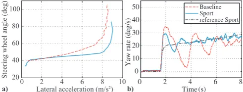
responses of the vehicle (De Novellis et al., 2012) and, thus, the creation of fundamentally different driving modes. For example, a model-based design procedure is used in De Novellis et al. (2015b) to define sets of vehicle understeer characteristics at different longitudinal accelerations and the corre-sponding reference yaw rates (implemented in Layer 1, section 2.1.) that yield a sporty vehicle cornering behavior. That is, a Sport mode was de-signed to reduce the understeer gradient, extend the region of linear vehicle operation, and signifi-cantly increase the maximum lateral acceleration compared to the passive vehicle (Fig. 4a). The ac-tive safety benefits of the TV controller during highly-transient maneuvers are highlighted by the time history of the measured yaw rate during an extreme step steer test. Figure 4b shows that the controller allows a considerable reduction of the yaw rate oscillations and settling time. Hence, the vehicle behavior is more consistent and predictable so that driving in extreme conditions becomes eas-ier.

In order to exploit the full benefits of TV con-trol in a safe way in all possible driving conditions the road friction conditions need to be known or, at least, reasonably well estimated. Unfortunately, this is not a trivial task. As an alternative, the torque-vectoring algorithm can be coupled with sideslip control to create a more robust controller that shows consistent and safe performance nearly

Baseline Sport reference Sport

0 2 4 6 8

0 10 20 30 40 50

Time (s)

Yaw rate (deg/s)

0 2 4 6 8 10

20 40 60 80 100

Lateral acceleration (m/s2₎

Steering wheel angle (deg)

a) b)

Time (s)

24 25 26 27 28 29 30 31

Sideslip angle,

β

(deg)

-18 -16 -14 -12 -10 -8 -6 -4 -2 0 2

β_min

β_min β_min

= -5 deg = -10 deg = -15 deg

Figure 5. Vehicle sideslip angle during step steer tests with 100 deg of steering wheel angle amplitude at 90 km/h with three different predefined sideslip limits βmin (Lu et al.,

2016).

independent of the prevailing friction conditions (Lu et al., 2016). Also, the concurrent yaw rate and sideslip controller allows the vehicle to operate at specified sideslip angles to enhance active safety (Fig. 5). Conversely, the controller could be used to create a drift mode to improve the fun-to-drive aspect.

2.3 Energy-efficiency improvement

Owing to the actuation redundancy of EVs with multiple motors, TV control can be used to mini-mize the overall energy consumption without compromising vehicle dynamics characteristics. In particular, power losses in the drivetrain and due to tire slips (which become significant at high accel-eration levels) are major sources of energy con-sumption that can be influenced by the individual wheel torque control (Tjønnas et al., 2010, Chen & Wang, 2012, Pennycott et al., 2014). Considering the capabilities of the TV controller, the energy-efficiency can be improved in two ways:

 by distributing the traction/braking force and yaw moment demands of the high-level control-ler (section 2.1, Layer 2) among the wheels ac-cording to specific energy efficient control allo-cation (CA) strategies (section 2.1, Layer 3), see section 3.

 by defining reference understeer characteristics (section 2.1, Layer 1) that minimize energy losses, provided that vehicle handling behavior may be influenced, see section 4.

The combination of both ways is possible and should maximize the energy savings benefits of torque-vectoring control.

3 ENERGY EFFICIENT CONTROL

ALLOCATION

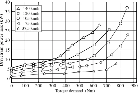
The energy efficient CA strategy implemented on the case study EV was developed based on meas-urements of the drivetrain power losses obtained on a rolling road facility. The power losses were determined from the difference between the ured electrical power at the inverter and the meas-ured mechanical power at the roller of the test bench so that the results include the losses in the electric motor drive, mechanical transmission, tire rolling resistance and tire slip on the roller. Figure 6 shows that the drivetrain power loss characteris-tics are strictly monotonically increasing functions of wheel torque with a single inflection point and vary with vehicle speed. Based on this observation, a simple, computationally efficient torque distribu-tion strategy for energy minimizadistribu-tion is possible.

By assuming small steering angles and consid-ering the basic vehicle geometry, the wheel torque distribution problem can be simplified by treating the two vehicle sides independently (Pennycott et al., 2014). That is, the torque demands correspond-ing to FX,C and MZ,C (section 2.1, Layer 2) for the left and right hand sides of the vehicle are given by:

, /

1 2

C Z

d L R

C

X M

F R

d

 _{ } _

   (1)

where d = half-track; and R = the wheel radius.

Using Equation (1), the developed energy effi-cient CA strategy (see details in Dizqah et al., 2016) employs a single drivetrain on each side of the vehicle when the respective torque demand on the left/right vehicle side (τd,L/R) is lower than a specified switching value τd,SW. Conversely, if the side torque demand is greater than τd,SW an even front-to-rear torque ratio on the particular side is

0 100 200 300 400 500 600 700 800 900

0 5 10 15 20 25 30 35 40

Torque demand (Nm)

D

riv

etra

in

p

o

w

er

lo

ss

(k

W

)

37.5 km/h 75 km/h 105 km/h 120 km/h 140 km/h

0 20 40 60 80 100 120 140 250

300 350 400 450 500 550 600 650

Speed (km/h)

S

w

it

ch

in

g

torq

u

e (N

m

)

Figure 7. Switching torque for one vehicle side at different vehicle speeds.

used. To guard against drivability issues, the tran-sition between the two torque distribution cases is smoothened with a sigmoid function.

The switching torque (Fig. 7) can be obtained offline by considering that the drivetrains of the case study EV have equal power losses Ploss. Then,

τd,SW is found from the condition when the power loss of using only a single drivetrain is equal to the power loss of using an even distribution:

Ploss (τd,SW, Θ) + Ploss (0, Θ) = 2Ploss (0.5 τd,SW, Θ)

(2)

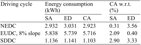
The CA was experimentally tested on the vehicle demonstrator by completing different driving cy-cles on the rolling road and comparing the results with tests of the EV set up with either front-wheel-drive (Single Axle, SA) or four-wheel-front-wheel-drive (Even Distribution, ED) with constant 50:50 front-to-rear wheel torque distribution. The tested driving cycles included the New European Driving Cycle (NEDC) to simulate low to medium driving loads, and the Extra Urban Driving Cycle (EUDC) run with an emulated uphill constant road slope of 8% to replicate medium to high driving loads. For both driving cycles, the CA strategy yields the lowest energy consumption, see Table 1. In terms of the NEDC, the potential energy improvement of the CA is rather small (<1%) with respect to the SA mode, whereas substantial improvements (>2.9%) are achieved compared to the ED mode.

Table 1. Energy consumption along driving cycles.

Energy consumption (kWh)

CA w.r.t. (%) Driving cycle

SA ED CA SA ED

NEDC 2.932 3.031 2.923 0.31 3.56

EUDC, 8% slope 5.838 5.739 5.716 2.09 0.40

SDDC 1.136 1.141 1.103 2.90 3.33

0 50 100 150 200

0 20 40 60 80 100 120 140

Time (s)

S

pee

d (

k

m

/h)

Figure 8. Speed profile of the SDDC.

This behavior can primarily be ascribed to the relatively low drive torque required during the NEDC compared to the motor torque available on the case study EV, so that τd,L/R < τd,SW is often true and the SA mode is close to being the most effi-cient torque distribution. This observation is con-firmed by the greater energy savings achieved rela-tive to the ED mode, and by the reversed trend for the EUDC with 8% slope, which requires a greater drive torque. In other words, an electric vehicle with less powerful drivetrains would show benefits more clearly in the two driving cycles. Thus, to emphasize the effect of the CA on energy con-sumption, a new driving cycle was created, it is called the Surrey Designed Driving Cycle (SDDC), see Figure 8. Over the SDDC, the CA algorithm is significantly better than the SA and ED modes, improving energy efficiency by 2.9% and 3.3%, respectively.

The concept of the simple, yet effective CA for-mulation is also valid during cornering and allows the car to operated with 2, 3 or 4 active motors. Tests of running the car at constant radius and ve-locity on a skid-pad showed energy consumption improvements of up to ~4% compared to the ED mode.

4 ENERGY EFFICIENT REFERENCE

UNDERSTEER CHARACTERISTIC

0 2 4 6 8 35 40 45 50 55 60 65 70 S tee ri n g wh eel a n g le ( d eg )

Lateral acceleration (m/s2₎

2 3 4 5 6 7 8

-2 -1 0 1 1.5 -1.5 0.5 -0.5 2

Lateral acceleration (m/s2₎

Yaw m o m en t ( k Nm ) PV U1 U2 U3 U4 U5 O1 O2 O3 O4 O5 a) b)

Figure 9. a) The experimentally measured understeer characteristics with different reference yaw moment settings. b) Reference yaw moment as a function of lateral acceleration for different understeer characteristics. The open black squares indicate the passive vehicle.

2 3 4 5 6 7 8

35 40 45 50 55 60 65

Lateral acceleration (m/s2₎

S te er ing w h ee l ang le ( de g ) 5 5 5 5 5 5 5 5 5 5 5 5 5 9 9 9 9 9 9 9 9 1317 5 5 5 5 5 5 5 5 5 5 5 5 9 9 9 9 9 9 9 9 9 1₃ 17 13 5 9 13 17

2 3 4 5 6 7 8

-2 -1.5 -1 -0.5 0 0.5 1 1.5 2 Ya w mo me n t (k Nm) R el at ive pow er i nput i ncr ea se ( % )

Lateral acceleration (m/s2₎

a) b)

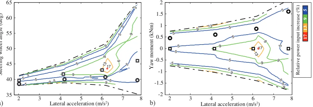
Figure 10. a) Map of understeer characteristics with iso-contour lines of relative drivetrain power increase with respect to the vehi-cle with the optimal understeer characteristic (indicated by black open cirvehi-cles). The passive vehivehi-cle understeer characteristic is shown by the black open squares and the boundaries of the measured region are indicated by the dash-dotted lines. b) Map of yaw moments with iso-contour lines of relative drivetrain power increase with respect to vehicle with optimal understeer characteristic. The optimum yaw moment is indicated by black open circles. The passive vehicle yaw moment is shown by the black open squares and the boundaries of the measured region are indicated by the dash-dotted lines.

one of the passive vehicle (denoted as PV), five characteristics with progressively increasing un-dersteer (denoted as U1 to U5) and five character-istics with progressively decreasing understeer (denoted as O1 to O5) with respect to the passive vehicle (Fig. 9a). The yaw moments corresponding to the different understeer characteristics are shown in Figure 9b. Positive yaw moments yield a destabilizing control action (reducing understeer) and negative yaw moments generate a stabilizing effect (increasing understeer).

For ease of comparison, the measured drivetrain power is expressed relative to the power required by the vehicle set up with the most energy efficient understeer characteristic, which is given by the steering wheel angle that minimizes P for a par-ticular lateral acceleration.

As indicated by Figure 10a, the optimal han-dling characteristic is achieved by reducing

under-steer compared to the passive vehicle. In particular, the most energy efficient cornering behavior is close to neutral steering, which is typically associ-ated with sports car characteristics and, thus, can be assumed to also enhance active safety and fun-to-drive aspects (see section 2.2). Over the meas-ured lateral acceleration range, the optimal under-steer characteristic allows energy savings of up to ~11% compared to the passive vehicle. This poten-tial saving is considerably greater than the im-provements achievable with the CA algorithm (see section 3). Also, it is expected that running the ve-hicle with the CA algorithm and the optimal un-dersteer gradient should yield further energy effi-ciency improvements.

positive and monotonically increasing with aY. In-terestingly, the relative power contours are nearly symmetric about the x-axis. Current work is con-cerned with this aspect.

5 CONCLUSIONS

The experimental work allows the following con-clusions:

 Torque vectoring control is effective in improv-ing energy efficiency by reducimprov-ing power losses associated with the drivetrain and tires.

 The energy efficient CA algorithm allows en-ergy savings typically between 2% and 3% along driving cycles and up to ~4% during cor-nering conditions with respect to fixed torque distribution strategies.

 The optimal understeer characteristic in terms of energy efficiency is close to the condition of neutral steering for the specific electric vehicle.

 The energy efficient reference cornering re-sponse reduces measured input power by up to ~11% for the case study vehicle demonstrator.

REFERENCES

Chen, Y., Wang, J. 2012. Fast and global optimal energy ef-ficient control allocation with applications to overactu-ated electric ground vehicles. IEEE Transactions Control

Systems Technology 20(5): 1202–1211.

Chen, Y., Wang, J., 2014. Adaptive energy-efficient control allocation for planar motion control of over-actuated elec-tric ground vehicles. IEEE Transactions Control Systems

Technology 22(4): 1362–1373.

De Novellis, L., Sorniotti, A., Gruber, P., Ivanov, V., Hoep-ping, K. 2012. Torque vectoring control for electric vehi-cles with individually controlled motors: state-of-the-art and future developments. In: 26th International Electric

Vehicle Symposium (EVS26), Los Angeles 6-9 May 2012.

De Novellis, L., Sorniotti, A., Gruber, P. 2013. Optimal wheel torque distribution for a four-wheel-drive fully electric vehicle. SAE International Journal of Passenger

Cars 6(1): 128–136.

De Novellis, L., Sorniotti, A., Gruber, P., Orus, J., Rodriguez Fortun, J.M., Theunissen, J., De Smet, J. 2015a. Direct yaw moment control actuated through electric drivetrains and friction brakes: theoretical design and experimental assessment. Mechatronics 26: 1–15.

De Novellis, L., Sorniotti, A., Gruber, P. 2015b. Driving modes for designing the cornering response of fully elec-tric vehicles with multiple motors. Mechanical Systems

and Signal Processing, 64-65: 1–15.

Dizqah, A. M., Lenzo, B., Sorniotti, A., Gruber, P., Fallah, S., De Smet, J. 2016. A Fast and Parametric Torque Dis-tribution Strategy for Four-Wheel-Drive Energy Efficient Electric Vehicles. IEEE Transactions on Industrial

Elec-tronics 63: 4367–4376.

Fujimoto, H., Harada, S. 2015. Model-based range extension control system for electric vehicles with front and rear driving-braking force distributions. IEEE Transactions on

Industrial Electronics 62(5): 3245–3254.

Jonasson, M., Andreasson, J., Solyom, S., Jacobson, B., Stensson Trigell, A. 2011. Utilization of actuators to

im-prove vehicle stability at the limit: from hydraulic brakes toward electric propulsion. Journal of Dynamic Systems,

Measurement, and Control 133(5): 051003.

Kang, J., Yoo, J., Yi, K. 2011. Driving control algorithm for maneuverability, lateral stability, and rollover prevention of 4WD electric vehicles with independently driven front and rear wheels. IEEE Transactions on Vehicular

Tech-nology 60(7): 2987–3001.

Lu, Q., Gentile, P., Tota, A., Sorniotti. A., Gruber, P., Co-stamagna, F., DeSmet, J. 2016. Enhancing vehicle corner-ing limit through sideslip and yaw rate control.

Mechani-cal Systems and Signal Processing 75: 455–472.

Pennycott, A., De Novellis, L., Sabbatini, A., Gruber, P., Sorniotti A. 2014. Reducing the Motor Power Losses of a Four-Wheel Drive Fully Electric Vehicle via Wheel Torque Allocation. Proceedings of the Institution of Me-chanical Engineers, Part D: Journal of Automobile

Engi-neering 228(7): 830–839.

Tjønnas, J., Johansen, T.A. 2010. Stabilization of automotive vehicles using active steering and adaptive brake control allocation. IEEE Transactions Control Systems Technol-ogy 18(3): 545–558.

van Zanten, A., Erhardt, R., Pfaff, G. 1995. VDC, the Vehi-cle Dynamics Control System of Bosch. SAE Technical

paper 950749.