Reversible polymorphism aware phylogenetic models and their application to tree inference

Reversible polymorphism-aware phylogenetic models and their

application to tree inference

Dominik Schrempf

a,b

, Bui Quang Minh

c

, Nicola De Maio

d,e

, Arndt von Haeseler

c

,

Carolin Kosiol

a,n

a

Institut für Populationsgenetik, Vetmeduni Vienna, Wien, Austria b

Vienna Graduate School of Population Genetics, Wien, Austria c

Center for Integrative Bioinformatics Vienna, Max F. Perutz Laboratories, University of Vienna, Medical University of Vienna, Austria d

Nuffield Department of Medicine, University of Oxford, UK e_{Oxford Martin School, University of Oxford, UK}

H I G H L I G H T S

Species tree inference from genome-wide population data. Takes incomplete lineage sorting into account.

Analytical solution of stationary distribution and formal proof of reversibility. Reversibility ensures swiftness and stability.

Increase of sample size per species improves estimations without raising runtime. Comparison to the Wright-Fisher diffusion.

a r t i c l e i n f o

Article history: Received 11 April 2016 Received in revised form 25 July 2016

Accepted 27 July 2016 Available online 29 July 2016

Keywords: Species tree Phylogenetics

Incomplete lineage sorting Substitution model

Reversible polymorphism-aware phyloge-netic model

a b s t r a c t

We present a reversible Polymorphism-Aware Phylogenetic Model (revPoMo) for species tree estimation from genome-wide data. revPoMo enables the reconstruction of large scale species trees for many within-species samples. It expands the alphabet of DNA substitution models to include polymorphic states, thereby, naturally accounting for incomplete lineage sorting. We implemented revPoMo in the maximum likelihood software IQ-TREE. A simulation study and an application to great apes data show that the runtimes of our approach and standard substitution models are comparable but that revPoMo has much better accuracy in estimating trees, divergence times and mutation rates. The advantage of revPoMo is that an increase of sample size per species improves estimations but does not increase runtime. Therefore, revPoMo is a valuable tool with several applications, from speciation dating to species tree reconstruction.

&2016 The Authors. Published by Elsevier Ltd. This is an open access article under the CC BY-NC-ND license (http://creativecommons.org/licenses/by-nc-nd/4.0/).

1. Introduction

Molecular phylogenetics seeks to understand evolutionary phenomena such as speciation dynamics and biodiversity by es-timating evolutionary parameters at the species level. The re-construction of the species history gives insights into the basic mechanisms of biology. However, the topology of the species tree is not always clear, especially when phylogenies from different genomic regions (i.e., gene trees or genealogies) differ from each

other (Degnan and Rosenberg, 2006).

Statistical approaches to tree reconstruction such as maximum likelihood and Bayesian methods rely on substitution models (Tavaré, 1986). These models describe and quantify the prob-abilities of how sequences may evolve along a phylogeny. They are defined by an instantaneous rate matrix Q that contains the substitution rates between the different character states. For computational convenience, most substitution models are re-versible. That is, the process describing the evolution of the se-quence is independent of the direction in time. Reversibility is important in phylogenetics for tree inference from large data sets with many species because it simplifies the likelihood function (Yang, 2006, p. 34) and reduces the number of trees by a factor of

− l

2 3, wherelis the number of tips of the tree (Hein et al., 2004, p. Contents lists available atScienceDirect

journal homepage:www.elsevier.com/locate/yjtbi

Journal of Theoretical Biology

http://dx.doi.org/10.1016/j.jtbi.2016.07.042

0022-5193/&2016 The Authors. Published by Elsevier Ltd. This is an open access article under the CC BY-NC-ND license (http://creativecommons.org/licenses/by-nc-nd/4.0/). n_{Corresponding author.}

E-mail addresses:[email protected](D. Schrempf),

70). Finally, rate matrices of reversible substitution models have real eigenvalues (Kelly, 1979) which enable a fast and stable ei-gendecomposition during matrix exponentiation (Golub and Loan, 1996). Many software packages use reversible substitution models (e.g., HyPhy,Pond et al., 2005; PhyML,Guindon et al., 2010and MrBayes,Ronquist et al., 2012). RAxML (Stamatakis, 2014) and IQ-TREE (Nguyen et al., 2015) additionally offer efficient tree search algorithms for very large phylogenies.

Substitution models, when naively applied to species trees (concatenation methods, e.g.,Gadagkar et al., 2005), assume the species or population to befixed for a specific character state and do not account for effects on the population genetics level such as Incomplete Lineage Sorting (ILS;Maddison, 1997;Knowles, 2009). Incompletely sorted lineages coalesce deep in the tree and their coalescent events do not match the speciation events. The prob-ability of ILS is large and consequently tree reconstruction is

dif-ficult if the time between speciation events is short or if the ef-fective population size is large (Pamilo and Nei, 1988). The mul-tispecies coalescent model can be used to quantify the phyloge-netic distortion due to ILS. It simulates a coalescent process (Kingman, 1982) on each branch of the species tree and combines these separate processes when branches join together. This model predicts that for specific evolutionary histories the gene trees with highest abundance conflict the species tree topology (anomaly zone; Degnan and Rosenberg, 2009; Degnan, 2013). These are extreme cases where common tree inference methods not ac-counting for ILS such as concatenation (Gadagkar et al., 2005) or democratic vote (Pamilo and Nei, 1988) fail because they are sta-tistically inconsistent (e.g.,Ewing et al., 2008). However, ILS con-siderably deteriorates estimates already when species trees are not in the anomaly zone (Pollard et al., 2006).

We have recently developed an approach calledPo lymorph-ism-Aware PhylogeneticModel (PoMo,De Maio et al., 2013). PoMo builds on top of substitution models but makes use of within-species data and considers present and ancestral polymorphisms thereby accounting for ILS. Similar to multispecies coalescent models it uses multiple sequence alignments of up to several hundred species while allowing for many within-species se-quences to infer base composition and mutational parameters. Recently, we applied PoMo to infer species trees (De Maio et al., 2015). We showed in a large scale simulation study with various demographic scenarios and evaluation against other state-of-the-art methods like BEST (Liu, 2008),*BEAST (Heled and Drummond, 2010), SNAPP (Bryant and et al., 2012) and STEM (Kubatko et al., 2009) that PoMo is approximately as fast as standard DNA sub-stitution models while being more accurate in terms of the branch score distance (Section 3.1). Furthermore, application to great apes data leads to phylogenies consistent with previous literature and also with the geographic distribution of the populations.

Here, we prove the reversibility of PoMo when an associated reversible mutation model (Section 2.3) is used and derive the corresponding stationary distribution. This will open the PoMo approach to a new area of applications because a reversible model can take advantage of existing algorithms that efficiently reconcile the species tree. We will discuss the reversible solution of PoMo, provide connections to the diffusion equation and introduce an implementation in IQ-TREE (Nguyen et al., 2015).

Finally, we present a simulation study and an application to real data to demonstrate the performance of the reversible PoMo (re-vPoMo) and to confirm its relevancy in medium-to-large-scale tree search.

2. Materials and methods

2.1. DNA substitution models

DNA substitution models assume that a DNA sequence evolves as a series of independent substitution events which replace a nucleotide by another one. Substitutions are modeled as a time-continuous, time-homogeneous Markov process (Yang, 1994). Additionally, the different sites of a sequence are assumed to evolve independently. The four nucleotidesA C G, , andTform the alphabet (. The rates of changeqxyfrom nucleotidexto

nucleo-tide y are summarized in an instantaneous rate matrix

= ( ) ∈

Q qxy x y, ( which completely describes the time-continuous

Markov process. The assumption of time-homogeneity implies that the entries ofQ are constant in time. One also assumes sta-tionarity, i.e., the existence of a stationary distribution π= (πx x)∈(

which is the solution toπQ=0. If the Markov process is reversible, then detailed balanceπ_{x xy}q =π_{y yx}q is fulfilled. Thus, for the General Time Reversible (GTR,Tavaré, 1984) model the rate matrix has the following structure:

⎛

⎝ ⎜ ⎜ ⎜ ⎜

⎞

⎠ ⎟ ⎟ ⎟ ⎟

π π π

π π π

π π π

π π π

= *

* *

* _{( )}

Q

A C G T

A C G T

r r r

r r r

r r r

r r r

,

1 AC C AG G AT T

CA A CG G CT T

GA A GC C GT T

TA A TC C TG G

with qxy=πy xyr and exchangeabilities rxy=ryx >0. The diagonal

entries are chosen such that the row sums are zero. The expected number of events on a branch of lengthdis ( ) = −d d∑_xπ_{x xx}q . Usually, Q is normalized such that ∑ ∑_{x x y≠} π_{x xy}q =1or( ) =1 1.

2.2. The alphabet of revPoMo

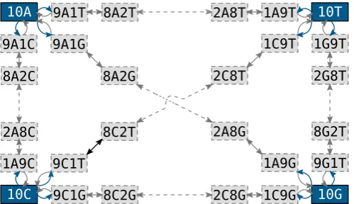
Standard DNA substitution models are limited in the sense that they assume that species are alwaysfixed for a specific nu-cleotide (i.e., the changes are substitutions). For revPoMo, we use standard DNA models such as HKY (Hasegawa et al., 1985) or GTR (Tavaré, 1984) as mutation models introducing variation into populations that are no longer assumed to befixed for one nu-cleotide. We expand the alphabet to include characters that re-present polymorphisms so that populations can have poly-morphic states. Thereby, revPoMo introduces a virtual haploid population of constant size Nand distinguishes between fixed (boundary) {Nx} = {Nx, 0y} = {0 ,y Nx} and polymorphic char-acters{ix N,( − ) }i y (1≤i≤N−1;x y, ∈ {A C G T, , , };x≠y), where

x and y are the nucleotides of the associated mutation model (Fig. 1). For convenience, we call the set of boundary characters theboundary. To keep the alphabet of revPoMo (PoMo

manage-able, we assume that at most two different nucleotides per site are present simultaneously. This is only a mild restriction and many real data sets meet this assumption. For example, no sites with three or four nucleotides have been found in the great apes data set described in Section 2.11. This restriction also agrees with the chosen mutation model (Section 2.3). The alphabet-size of revPoMo is

⎜ ⎟

⎛ ⎝

⎞ ⎠

| | = + ( − )

( ) N

4 4

2 1 . 2

PoMo (

To differentiate between revPoMo and the associated mutation model, we refer to the characters of the mutation model as nu-cleotides and to the characters of revPoMo as states. The in-stantaneous rate matrix of revPoMo QrevPoMo is composed of the

rates of mutations and genetic drift

= + _{( )}

which will be discussed in the next two sections.

2.3. The mutation model of revPoMo

For any nucleotide pair (x,y) with x≠y, the state {Nx}can mutate to state {(N−1 , 1)x y}at rate

μxy

introducing a new nu-cleotideyinto the population. Additionally to restricting the state space, mutations are confined to the boundary only. This is a good assumption if mutation rates are low or if genetic drift removes variation reasonably fast (Vogl and Clemente, 2012), a requirement that is met for low effective population sizes. Analogous to the GTR model, the mutation coefficients

μxy

can be decomposed into

μxy=mxy yπ, wheremxy=myxand

πy

is the entry of the stationary

distribution of the mutation model corresponding to nucleotidey. Although the concepts are similar we separate the substitution rates from the mutation rates of the associated mutation model by using different symbols (qxy∼μxy,rxy∼mxy). The symmetry of the

coefficients mxy is a requirement for the reversibility of the GTR

model and consequently also of revPoMo. This type of mutation model alsofits the structure of the alphabet of revPoMo which only allows two nucleotides to be present in a virtual population. The mutation rates

μxy

of the associated mutation model are summarized in the rate matrixQMutof dimension|(PoMo|. All other

rates are zero and the diagonal elements are defined such that the respective row sum is zero.

2.4. Genetic drift in revPoMo

The drift rate for a polymorphic state is modeled with the time-continuous neutral Moran model (e.g.,Durrett, 2008, p. 46). Given a virtual population of sizeN, in each generation an individual is randomly chosen to reproduce. The offspring is of the same type as the parent and replaces another randomly chosen individual from the population. Thereby, the population size remains constant. For

≤i≤N−

1 1, the rate of change from a state{ix N,( − ) }i y to states

{( +i 1 ,)x N( −i−1) }y or{( −i 1 ,)x N( −i+1) }y is

= = = ( − )

( )

+ −

q q q i N i

N . 4

i i, 1 i i, 1 i

Similar to the mutation model, these rates are summarized in the rate matrix Q_Drift of dimension |(PoMo|. Again, all other rates are

zero and the diagonal elements are determined by the require-ment that all row sums are zero. For our polymorphic states, the model is symmetric because the rates of increase and decrease are

equal. Importantly, nucleotide frequency shifts larger than one require more than one drift event (Fig. 1). In contrast to DNA substitution models, a substitution in revPoMo is the interplay of a mutational event with subsequent frequency shifts such that the newly introduced nucleotide becomesfixed.

2.5. Reversibility of revPoMo

If the equilibrium of a Markov process exists it is described by the stationary distributionπ(see above). The stationary distribu-tion of the time-continuous Markov process defined by the in-stantaneous rate matrixQrevPoMo(Appendix A)will be denotedpto

differentiate it from the stationary distribution of the Markov process of the associated mutation model π. The entries corre-sponding to the four boundary states are denoted px, the entries

corresponding to polymorphic states {ix N,( − ) }i y (1≤i≤N−1,

≠

x y) are pxyi. The number of elements of pis|(PoMo|(Eq.2). Theorem 1. The Markov process defined by QrevPoMo is reversible with stationary distribution

π

= ( )

px c x, 5

π π

= _{( )}

p_xyi c m / .q ₆

x y xy i

The normalization constant is

⎛

⎝ ⎜ ⎜ ⎜

⎞

⎠ ⎟ ⎟ ⎟

∑

∑

π π

= +

( ) =

−

∈ ≠

−

c

k m

1 1 .

7 k

N

x y x y

x y xy 1

1 ,

1

(

Note that ∑_kN₌−₁11/k is half of the expected branch length of a genealogy withNsamples for the standard coalescent model. This coincides with the rate of coalescence in the Moran model being twice as much as the rate in the standard coalescence model. Furthermore,∑_{x y},_∈(,_{x y≠} π πx ymxy is the expected number of

muta-tions per site and unit time for the associated mutation model.

Proof. An irreducible Markov process with a finite number of states is reversible if its (unique) stationary distribution fulfills detailed balance p qr rs=p qs sr (r s, ∈(PoMo; e.g., Norris, 1998, p.

125). We distinguish two cases: (a) balance between boundary states and their neighbors

μ

{Nx} ⇌ {(N− )1 , 1x y}: p_{x xy}=p q_xy1 1 _{( )8}

and (b) balance between neighboring polymorphic states

{_{ix N,}( − ) } ⇌ {( + )_{i y i 1 ,x N}( −_i− ) }_{1y : p q} =_p+_q+_{, ( )} 9 xy

i i xy i 1 i 1

where 1≤i≤N−2. Both conditions can be verified using Eqs.

(5)and(6). Supplemental Section S1 shows the derivation of the normalization constant and the computation of the stationary distribution p. □

2.6. The stationary distribution

In this section we illustrate the stationary distribution p of revPoMo and connect it to previous results of phylogenetics and population genetics. Similarly to DNA substitution models, the frequencies of the boundary statespxare proportional to the

[image:3.595.35.285.57.201.2]

sta-tionary distribution of the nucleotides π. revPoMo can estimate this nucleotide distribution empirically from the alignment data or by maximum likelihood. We were concerned that the genetic variation at stationarity of the small, virtual population of re-vPoMo represented bypxyidiffers considerably from the genetic

Fig. 1.The alphabet of revPoMo and its connectivity forN¼10. Blue and gray ar-rows indicate mutations and genetic drift, respectively. Dashed arar-rows symbolize the presence of intermediate states. A virtual population that is in the boundary state{10A}can move to the polymorphic states{9 , 1A C}, {9 , 1A G}and{9 , 1A T}

through a mutational event. Only states with frequency changes of size one are directly connected. For example, two jumps of the Markov process are needed to move from{10A}to{8 , 2A G}. (For interpretation of the references to color in this

variation in the real (modeled) populations with high effective population sizes. A substantial amount of theoretical work exists that models the dynamics and the equilibrium properties of po-pulations assuming very large effective population sizes (diffusion limit; e.g.,Wright, 1931,1945;Kimura, 1964). The diffusion limit has been found to be an adequate approximation in a broad range of population genetics scenarios (Kimura, 1964). We compared the polymorphic entries of the stationary distribution of revPoMopxyi

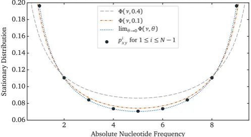
to the stationary solution of the diallelic diffusion equation with drift, equal mutation rates and without selection (e.g., Durrett, 2008, p. 254) which is the probability density of the Beta dis-tribution Φ ν θ( , ) ∼Beta ,(θ θ), where

ν

is the continuous allele frequency. It converges to

ν( − )ν 1

1 if the scaled mutation rate θ=4Neμ is small. The elements of the stationary distribution of

PoMo corresponding to polymorphic states pxyi are distributed

proportional to its discrete, empirical version

( − ) i N i

1 _{(Fig. 2). In}

particular, revPoMo is a good approximation ifθ<0.1. Many real data sets (e.g., genomic sequences of mammals, andDrosophila

species) meet this requirement. For microbial data sets, however, this assumption might not be valid. Section S2 includes additional thoughts on the stationary distribution for non-uniformπ.

2.7. Number of parameters

This section discusses a peculiarity of the number of para-meters of revPoMo compared to the associated mutation model. For example, both the GTR model and revPoMo with the GTR model as associated mutation model (GTR_þrevPoMo) have three free parameters for the stationary nucleotide frequencies because the four entries of πhave to sum to one. Furthermore, the GTR model normalizes the substitution coefficients such that the total substitution rate is one per unit time, i.e.,

∑

π

∑

π π

− = =

( )

∈ ∈

≠

q r 1.

10 x

x xx x y

x y x y xy ,

( (

Thereby it reduces the number of free rate parameters from six to

five. This step is necessary because only the ratios of the sub-stitution coefficients matter and the total substitution rate be-tween nucleotides is confounded with the branch lengths. How-ever, in revPoMo the total rate of mutations cannot be constrained in the same way because it also determines the percentage of polymorphic states in the stationary distributionp(Eq.7). Scaling the symmetric mutation coefficients mxy by a common factor

affects the ratio p px/ xy

i _{. This is why the number of parameters of}

revPoMo is larger by one, e.g., the GTR model has eight and GTRþrevPoMo has nine parameters. Previously, this additional unknown variable was empirically estimated (De Maio et al., 2013). In contrast, we jointly infer it with all other model parameters.

2.8. Relation between revPoMo and substitution models

It is desirable to compare distance estimations of revPoMo with estimations from standard DNA substitution models. We have seen, however, that a mutation from the boundary requires sub-sequent nucleotide frequency shifts to become a substitution and that the total number of mutations scales with phylogenetic dis-tance. Phylogenetic distances are usually normalized such that on average one event (i.e., one jump of the Markov process) happens per unit length (see alsoSection 2.7). If a Markov process starts in equilibrium, we have(# ) =E d, where#Eis the number of events

anddis the total branch length. For substitution models, the ex-pected number of substitutions is (# ) =S (# ) =E d. Also in

re-vPoMo the total rate of events per unit length can be normalized to one. However, events can still be either mutations or frequency shifts. Let mbe the probability that an event is a mutation. This mutation moves away from a boundary state{Nx}towards a dif-ferent nucleotidey. Lethbe the hitting probability of the opposite boundary state {Ny}before moving back to {Nx}.hdoes not de-pend onxandy because revPoMo assumes boundary mutations only. The expected number of substitutions is

(#S revPoMo, ) =(# )E mh. (11)

From population genetics, we know that h=1/N (e.g. Ewens, 2004, p. 105) because genetic drift is the only active force and the frequency ofyis just1/N. A comparison of the transition rates of

QrevPoMoshows that also m=1/N(Appendix B)and we get

(# ) =

( )

d

N . 12

S revPoMo, ₂

This enables us to compare the branch lengths of revPoMo with the ones of standard DNA substitution models if we assume that the estimated number of substitutions (# )S and (#S revPoMo, )are

equal across both models.

2.9. Implementation

We present an implementation of revPoMo in IQ-TREE (Nguyen et al., 2015; for technical details see Section S5). We allow the virtual population sizeNto vary between 2 and 19. The maximum of 19 is an arbitrarily chosen cut-off to keep the size of the ex-ecutable small. revPoMo uses multiple sequence alignments in the form of countsfiles as input data (De Maio et al., 2015). That is, nucleotide counts are given for each site and population. In gen-eral, the nucleotide counts (i.e., the number of sampled individuals from a population) will differ from the virtual population sizeNof revPoMo. Furthermore, sequencing errors, merged data from dif-ferent sources as well as alignment problems may lead to a var-iation of nucleotide counts between populations or even within populations at different sites. In contrast to DNA substitution models, where the character of the corresponding terminal node is set to the observed nucleotide, the revPoMo state at the same terminal node is not obvious anymore if the sample size is not equal toN. A simple method to determine the revPoMo state is to sampleNnucleotides with replacement from the given data. We do this independently for each site and population and call this methodsampled.

[image:4.595.44.293.536.672.2]

Instead, similarly to handling ambiguity and error (Felsenstein,

Fig. 2.A comparison of the stationary solution of the diffusion equation (Wright, 1931)Φ ν θ(_, ) =νθ−1.0(₁− )νθ−1.0_{for equal scaled mutation ratesθ=4N ue and drift} with the polymorphic elements of the stationary distribution of revPoMo forN¼10. νis the continuous relative nucleotide frequency. Both pandΦhave been nor-malized such that the polymorphic elements integrate to one and the domain ofΦ has been expanded from(0, 1)to(0, 10).Φconverges to a continuous version of pxyi

2004, p. 255), we can also weight the revPoMo states at each terminal node according to their likelihood of representing the observed counts. We set these likelihoods to the binomial dis-tribution because a revPoMo state represents a real population with the same proportions of nucleotides. In detail, for a terminal node with observed nucleotide counts{jx M,( − ) }j y, the likelihood of revPoMo state{ix N,( − ) }i y is

 ⎛

⎝ ⎜⎜ ⎞

⎠

⎟⎟⎛_⎝⎜ ⎞_⎠⎟ ⎛_⎝⎜ ⎞_⎠⎟( )

({ ( − ) }|{ ( − ) }) = −

( )

−

jx M j y ix N i y M

j i N

N i

N

, ,

13

j M j

⎛ ⎝

⎜ ⎞

⎠ ⎟ =

( )

j M i

N Bin ; , ,

14

where0≤j≤Mand0≤i≤N. Only nucleotides that are present in the virtual population can be sampled. We call this sampling methodweighted.

2.10. Simulation study

The performance of revPoMo was tested with simulated se-quences. Two different pipelines were used to create genealogies. First, for scenarios with four (e.g.,Fig. 3) and eight extant species, the species trees were prede_fined and genealogies were simulated with the coalescent simulation program MSMS (Ewing and Her-misson, 2010). For the coalescent simulations, the tree height is specified in units of effective population sizeNe. We used values of

N

1 eand10Ne. Between two and twenty individuals were sampled

per population. That is, the genealogies for the scenarios with four taxa have up to 80 tips. Second, in the larger scenario with 60 species, the species trees were created under a Yule birth model (Yule, 1925). A new species tree was simulated for each replicate. We used SimPhy (Mallo et al., 2016) to simulate the species tree and subsequently the genealogies with 10 individuals per popu-lation. Overall, these genealogies have 600 tips. The tree height wasfixed to 3Ne and the parameter describing the rate of

spe-ciations events per coalescent time unit was determined such that the expected coalescence time for 60 species matches 3Ne. This

corresponds to a rate of 1.226 speciations perNe.

For both pipelines 1000 independent genealogies were simu-lated. We used these genealogies to generate DNA sequences of

genes with Seq-Gen (Rambaut and Grass, 1997) using the HKY model. Thereby, we scaled the branch lengths with a factor of 0.0025. In particular, for scenarios with tree height 1Ne, the

number of substitutions per site from the root to the tips is 0.0025 on average. Likewise, the level of polymorphism within a species was equal for all scenarios and corresponds to an average Wat-terson's theta (Watterson, 1975) of 0.0025 per site. The sequence or gene length per genealogy was set to 1000 base pairs (bp). This simulation procedure is equivalent to no recombination within genes, free recombination between genes and no migration be-tween species. The amount of input data was varied bebe-tween three and all 1000 genes. We performed 10 replicate analyses for each setting. In the main text, we include results for theIncomplete Lineage Sortingspecies tree scenario (Fig. 3;DeMaio et al., 2015) and Yule trees with 60 species. A calculation according to the multispecies coalescent model shows that for the incomplete lineage sorting scenario, if one gene is sampled out of each species

A,BandC, about 55% of the genealogies that connect these genes are expected to exhibit ILS.

The analysis of the simulated data focuses on the comparison of three different methods: (1) a standard concatenation approach, where the input sequences within species are concatenated and a DNA substitution model is used for the analysis, (2) the non-re-versible PoMo with N¼10 implemented in HyPhy (Pond et al., 2005;De Maio et al., 2015) and (3) the new reversible version with varying N and weighted sampling implemented in IQ-TREE (Nguyen et al., 2015). All methods use the HKY substitution model (Hasegawa et al., 1985).

The accuracy of the estimation was measured with the branch score distance (BSD,Kuhner and Felsenstein, 1994) between the true and the estimated species tree. The BSD is the square root of the sum of the quadratic differences in branch lengths between two trees. For one taxon trees it coincides with the relative branch length error. Branches that do not exist in both trees due to dif-ferences in topology fully contribute to the BSD. Before we calcu-lated BSDs with PHYLIP (Felsenstein, 2005), the trees were nor-malized such that their total branch lengths equal 1.0. Normal-ization is necessary because branch lengths are confounded with substitution rates for DNA substitution models and have a different meaning for PoMo (Section 2.8). Sections S3 and S4 provide com-mand lines for the simulation and analysis procedure, respectively.

2.11. Application to great apes

Shared ancestral polymorphisms are very common in great apes (Dutheil et al., 2009). A variety of evolutionary patterns, short internal branches as well as closely related taxa lead to a high level of incompletely sorted lineages between Humans, Chimpanzees and Gorillas (about 25%,Scally et al., 2012). We apply revPoMo to a data set that includes all 6 great apes species divided into 12 po-pulations (Prado-Martinez et al., 2013). The number of sequences per population varies highly between 1 (Gorilla gorilla diehli) and 23 (Gorilla gorilla gorilla). About 2.8 million exome-widely dis-tributed, 4-fold degenerate sites were analyzed. We use the sam-pled input method which may lead to differences in estimates between runs. We do not expect a high divergence between runs but asses the variance by doing 10 replicate analyses.

3. Results and discussion

3.1. Simulations

[image:5.595.63.257.515.701.2]

A previous simulation study showed that the non-reversible PoMo outperforms other state-of-the-art methods (De Maio et al., 2015) in estimating species trees from large data sets. To begin

Fig. 3.TheIncomplete Lineage Sorting(ILS) scenario is a species tree with four tips and height 1Ne, whereNeis the effective population size. The lengths of

with, we assay the speed of the concatenation method, the non-reversible PoMo and revPoMo for different amounts of sequence data (in number of genes, one gene has 1000 bp). The introduction of reversibility improves speed greatly and the new implementa-tion of revPoMo in IQ-TREE runs up to 50 times faster than the version implemented in HyPhy. Overall, the runtime is similar to that of standard DNA substitution models (Fig. 4and Section S6 with Figs. S1–S3).

The simulation scenario with four species exhibits a significant amount of ILS and both PoMo approaches outperform the con-catenation method if the input data contains enough in-dependently evolved genes (Fig. 5). At least 50 genes (50k bp) are needed to get trustworthy results with small standard deviations and analyses of 1000 genes have an error of about 2% only. In general, the error is small (Section S7 and Figs. S4–S18). For species trees that do not exhibit any incomplete lineage sorting, the ac-curacy of PoMo measured in BSD is similar to the one from con-catenation methods and slightly better if more than three samples per population and about 50 genes are available (e.g., Sections S7.3 and S7.4 but alsoDe Maio et al., 2015).

With the non-reversible version of PoMo we were limited to trees of about a dozen species only. revPoMo takes advantage of efficient algorithms and the reduced runtime enables us to analyze

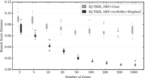
trees with many species. Here, we present an analysis of trees with 60 species generated under the Yule birth model. The non-re-versible PoMo approach is too slow for trees of this size. The runtime of revPoMo on sequences with 1000 genes is about 4.5 h with a standard deviation of about 25 min (i5Sunderland, MA, 2.70 GHz, 2 physical cores). Taking polymorphisms into account improves accuracy in terms of BSD for this scenario. In particular, if more than 100 independently evolved genes are used for the analysis, the BSD is reduced by a factor of seven (Fig. 6). Notably, revPoMo performs better than concatenation methods already if three genes are available. Although it is expected that an increase in the number of species leads to a higher chance of topological errors, the total error is similar to the one of the ILS scenario with four species only. Section S7.5 includes results for a Yule tree with 50 species.

A very important variable of PoMo is the virtual population size

Nwhich has initially been set to 10 for parameter estimation (De Maio et al., 2013). Up to this point, only the weighted sampling method has been used. Now we use both sampling methods

sampled and weighted to analyze the ILS scenario with 10 se-quences per species and 1000 genes in dependence ofN. Wefind that the allowance of a single polymorphic state for each pair of bases (N¼2) already decreases the tree estimation error and that an increase ofNfrom two to nine greatly improves the accuracy (Fig. 7). During a further increase ofNup to 19 the improvement is only marginal. Random sampling with replacement ofNsamples from the data gives better results ifNis very low. For higher virtual population sizes between 5 and 15, weighting the partial like-lihoods performs better on average and is also numerically more stable. Values of Nabove the sample size do not add useful in-formation and therefore do not positively influence the performance.

Additional results (Section S8 and Fig. S20–S24) confirm that for the weightedsampling method an increase of the virtual po-pulation size above the sample size does not greatly improve the results. For the sampled input method andNabove 10, we also observed numerical underflow errors due to low frequencies of polymorphic states of the stationary distribution if the alphabet is oversized. In general, we advice to choose N between 5 (large trees) and 19 (small to intermediately sized trees), depending on computational resources, tree size and input data. The sampled

input method seems to do better if the average number of samples is below three.

[image:6.595.44.293.318.451.2]

The total branch length of the inferred phylogeny is a further

[image:6.595.45.294.539.673.2]

Fig. 4.A boxplot of the runtimes of the concatenation approach (IQ-TREE, HKYþConc), the non-reversible PoMo withN¼10 (HyPhy, HKYþPoMo) and re-vPoMo with N¼10 and the weighted sampling scheme (IQ-TREE, HKYþrevPoMoþWeighted) for the ILS scenario with 10 samples and a tree height of1Ne(Fig. 3). The HKY model was used for all methods. Ten replicate analyses were performed. Different amounts of input data are shown on thex-axis (each gene has a length of 1000 bp).

Fig. 5.Tree error measured by the branch score distance for concatenation (IQ-TREE, HKYþConc), the non-reversible PoMo withN¼10 (HyPhy, HKYþPoMo) and revPoMo with N¼10 and the weighted sampling scheme (IQ-TREE, HKYþrevPoMoþWeighted) in dependence of the amount of data; one gene has 1000 bp. The HKY model was used for all models. The analyzed sequences were simulated under the ILS scenario with 10 samples and a tree height of 1Neor 0.0025 substitutions per site (Fig. 3). The non-reversible version performs mar-ginally better because the frequency distribution at the root is arbitrary.

Fig. 6. Branch score distance for the concatenation approach (IQ-TREE, HKYþConc) and revPoMo with N¼9 and the weighted sampling scheme (IQ-TREE, HKYþrevPoMoþWeighted) applied to sequences simulated under a Yule tree with 60 species with 10 samples each. The HKY model was used in both cases. The tree height is 3Neand the level of polymorphism measured by Watterson's theta is θW≈0.0025per site. Ten replicate analyses were performed. Thex-axis denotes the

[image:6.595.314.562.547.681.2]

criterion to judge the quality of revPoMo. Usually, the branch lengths of phylogenies inferred by Markov process based models are given in units of estimated average number of events per site. The connection between mutation and substitution rates (cf. Methods) allows an interpretation of the estimated branch lengths of revPoMo. In particular, we can convert the branch lengths to

estimated average number of substitutions per site, compare them to estimations from standard substitution models and—for simula-tions—also to the true value (Fig. 8).

The concatenation approach systematically overestimates the phylogenetic distance because polymorphisms are interpreted as substitutions. For revPoMo, wefind that the estimated tree length in substitutions improves for both input methods ifNis increased. The sampled input method seems to converge faster but over-shoots for values ofNabove the sample size. The further decrease of branch lengths can be attributed to an unnecessary inter-pretation of substitutions as standing polymorphisms. We con-clude that it is only preferable to use thesampledinput method when the data contains populations with very few individuals.

3.2. Real data

The previous, non-reversible PoMo already performed well on the great apes data set (De Maio et al., 2015). The phylogeny es-timated by revPoMo (Fig. 9) agrees with the geographic distribu-tion of the great apes (species with neighboring habitats are more closely related than species that live further apart) and the to-pology presented in the original publication (Prado-Martinez et al., 2013). revPoMo evaluates all (weighted) or nearly all (sampled) available polymorphic information in the data and we expect that estimates between consecutive runs have no or low variance, re-spectively. Indeed, 10 replicate analyses with the GTR model ( Ta-varé, 1986), N¼9 and thesampled input method show that it is stable and accurate. The estimated topologies are identical and the total branch lengths have a mean of _{3.08 10}· −2 _{substitutions/site}

with a very low standard deviation of about _{6.45 10}· −7

substitu-tions/site. On the contrary, the topology inferred by DNA sub-stitution models is not stable and depends on the individuals chosen to represent the species (De Maio et al., 2015).

The branch lengths of revPoMo can be used to estimate the germline mutation rate per generation within the Human– Chim-panzee–Gorilla clade. This is interesting because many dis-crepancies of estimates have been discussed in the past (Scally and Durbin, 2012). We assume that Humans split from Chimpanzees 7 million years ago (Ségurel et al., 2014) and that the Human–

Chimpanzee clade split from the Gorilla clade 10 million years ago (Scally and Durbin, 2012). Furthermore, we set the generation time to 25 years. Then, we get an estimate of about_{2.65 10}· −8_germline

mutations per generation per site. This value lies on the lower boundary of other estimates from phylogenies (Li and Tanimura, 1987; Takahata and Satta, 1997). We stress that this is a rough estimate that ignores various complex aspects considered by Li and Takahata. However, with our approach we take into account the effect of standing and ancestral variation on the estimate of mutation rates.

4. Conclusions

[image:7.595.35.283.58.192.2]

Polymorphism-aware phylogenetic models have been shown to improve accuracy substantially in parameter estimation (De Maio et al., 2013) and tree inference (De Maio et al., 2015) in the pre-sence of ILS. However, the number of populations that could be

Fig. 8.The estimated tree length in substitutions per site in dependence of the virtual population sizeN for revPoMo with both sampling methods (IQ-TREE, HKYþrevPoMoþSampled; IQ-TREE, HKYþrevPoMoþWeighted). The analyzed scenario is incomplete lineage sorting with 10 samples, a tree height of1Neand 1000 genes of input data. The errors bars are hardly visible and denote standard deviations of 10 replicate analyses. The dashed line is the true value. ForN¼1, the estimate of the concatenation approach (IQ-TREE, HKYþConc) is shown.

[image:7.595.303.553.58.191.2]

Fig. 9.The estimated phylogeny of the great apes data set with revPoMo and the GTR model agrees with the geographic distribution of the species. There are no topological differences between the 10 replicate analyses. The virtual population size was set toN¼9 and the input method tosampled. The phylogenetic scale is in substitutions/site and can be directly compared to values inferred by standard substitution models.

[image:7.595.316.536.277.478.2]

analyzed with the non-reversible PoMo implementation was limited. Here, we present a reversible PoMo under the following assumptions: (a) polymorphic states can only contain two differ-ent nucleotides, (b) the associated mutation model is reversible, (c) drift is described by the continuous-time Moran model (e.g.,

Durrett, 2008, p. 46) and (d) mutations can only happen when a nucleotide isfixed in the population. The stationary distribution for polymorphic states mimics the stationary solution of the dif-fusion equation without selection and low scaled mutation rate

θ

. The number of free parameters of revPoMo is determined by the associated mutation model plus one for the total mutation rate which determines the proportion of polymorphic states. This ad-ditional parameter can also be empirically estimated from the data. A generalization of the mutation model such that mutations can happen anytime not only naturally demands a further ex-pansion of the alphabet of revPoMo to allow states with multiple nucleotides but also introduces problems with respect to reversi-bility. Because of the Kolmogorov criterion (Kelly, 1979, p. 21), the mutation coefficients themselves have to be symmetric then, i.e.,

=

qxy qyxand not only rxy=ryxin Eq.(1). This is incompatible with

mutation models that use estimates of nucleotide frequencies like the HKY model. Furthermore, for polymorphic states the sta-tionary distribution is symmetric with respect to an interchange of nucleotides (Section 2.4). It may be interesting to investigate if and only if this symmetry is implied by a reversible mutation model.

The introduction of reversibility slightly increases the error in tree inference for some scenarios that have been examined but greatly improves runtimes up to a factor of 50. This allows the reconstruction of large-scale phylogenies. As an example, a Yule tree with 60 species was analyzed and low error rates were ob-served. We confirm that revPoMo does well on real data and infers a phylogeny that agrees with the geographical distribution of the analyzed populations. We also presented how the branch lengths of phylogenies estimated by revPoMo can be interpreted and compared to the ones estimated by standard substitution models. Finally, we show how the introduction of polymorphic states and an increase of the virtual population sizeNimproves estimates. We advise to chooseNbetween 5 (large trees) and 19 (small to intermediately sized trees), depending on computational sources, tree size and input data. We discourage from using re-vPoMo on sequence data where no population data is available yet. Describing the evolution of DNA sequences with Markov pro-cesses is very fast but restricts the possibilities of revPoMo to include, e.g., a model of geneflow. However, we want to assess robustness against geneflow in the future. An extension that we would like to implement is the inclusion of rate variation, for example with a gamma distribution. Rate variation might not only be modeled be-tween sites but also along the tree, e.g., to account for changes in effective population size. In particular, it is of high interest to relate the virtual population size of revPoMo to the effective population size of real populations. This would allow direct inference of effective population size as well as germline mutation rates.

Two different methods to process the data at the leaves of the phylogenysampled and weighted were implemented. We found that both sampling schemes influence accuracy, especially when the sample size is low. With theweightedsampling method a beta-binomial distribution could be used to allow pool sequence ( Fut-schik and Schlötterer, 2010) input data with sequencing errors (Appendix S5.2). Furthermore, one could run a diffusion process that connects the data to the leaves to improve the determination of the likelihoods of the revPoMo states. This would also enable us to model population genetic effects with large or even variableNe

relatively close to the present which is the stage where these ef-fects are most important. We would also like to enable automatic bootstrap with IQ-TREE. Importantly, we want to stress that the

idea of revPoMo can be used with substitution models of any type including alphabets consisting of amino acids or codons.

revPoMo is peculiar in the sense that it is discrete in frequency but continuous in time. This property makes it a connection be-tween models that are discrete in time and frequency (e.g., Wright–Fisher model with mutations) and the diffusion limit which corresponds to continuity in time and frequency. The ad-vantage of revPoMo compared to multispecies coalescence based models is that an increase of sample size improves tree and parameter estimations but does not increase runtime. We believe that revPoMo is a valuable tool in species tree estimation from population data.

Acknowledgments

We thank Claus Vogl and Asger Hobolth for discussions and valuable comments about revPoMo. This work is supported by the Austrian Science Fund (FWF-P24551 and I-2805-B29) and partially by the Vienna Graduate School of Population Genetics (FWF-W1225).

Appendix A. The instantaneous rate matrixQrevPoMo

Letqij

xybe the rate of a jump from{ix N,( − ) }i y to{jx N,( − ) }j y .

We can summarize Q_revPoMoas

⎧

⎨ ⎪ ⎪

⎩ ⎪ ⎪ μ

μ =

| − | >

= =

= = −

< < | − | = _{( )}

q

i j

i j

i N j N

q i N i j

0 if 1,

if 0, 1,

if , 1,

if 0 and 1, 15

xy ij yx

xy

i

where

= = = ( − )

( )

+ −

q q q i N i

N 16

i i, 1 i i, 1 i

(Section 2.4), x≠y and the diagonal elements (q_xx00_orq xxNNand qxyii,0<i<N) are defined such that the respective row sum is 0.

Appendix B. Derivation of (#S revPoMo, )

This section derives the expected number of substitutions of revPoMo (Section 2.8). If we denotemto be the probability of an event to be a mutation, the expected number of substitutions is

(#S revPoMo, ) =(# )E mh. (17)

m is the ratio of the rate of mutations rm to the total rate

= +

r rm rs. We have

∑

π μ

∑

π π

= =

( )

∈ ≠

∈ ≠

r c c m ,

18 m

x y x y

x xy x y

x y

x y xy

, ( , (

⎡ ⎣ ⎢ ⎢ ⎢ ⎢ ⎤ ⎦ ⎥ ⎥ ⎥ ⎥

∑

∑

∑

∑

∑

∑

∑

π π =

= +

=

= ( − ) ( )

∈ ≠ < <

≤ ≤ ≠

∈ ≠ < <

− +

∈ ≠ < <

r p q

p q q

c m

r N r

1 2

1 2

1 , 19

s x y

x y i N j N j i xy i xy ij x y x y i N

xy i xy i i xy i i x y x y i N

x y xy

s m

, 0 0

, 0

, 1 , 1

, 0 (

(

(

where the q_xyij _{are the rates from {ix N,( − ) } → {i y jx N,( − ) }j y}

(_q + =_q − xy i i

xy i i

, 1 , 1_{; Section S1). Finally,}





= = ( + ) =

(# ) =

( )

r r r r r N

l N

/ / 1/ , and

.

20

m m m s m

S revPoMo, ₂

Appendix C. Supplementary data

Supplementary data associated with this article can be found in the online version athttp://dx.doi.org/10.1016/j.jtbi.2016.07.042.

References

Bryant, D., et al., 2012. Inferring species trees directly from biallelic genetic mar-kers: bypassing gene trees in a full coalescent analysis. Mol. Biol. Evol. 29 (8), 1917–1932.

De Maio, N., Schlötterer, C., Kosiol, C., 2013. Linking great apes genome evolution across time scales using polymorphism-aware phylogenetic models. Mol. Biol. Evol. 30 (10), 2249–2262.

De Maio, N., Schrempf, D., Kosiol, C., 2015. PoMo: an allele frequency-based ap-proach for species tree estimation. Syst. Biol. 64 (6), 1018–1031.

Degnan, J.H., 2013. Anomalous unrooted gene trees. Syst. Biol. 62 (4), 574–590.

Degnan, J.H., Rosenberg, N.A., 2006. Discordance of species trees with their most likely gene trees. PLoS Genet 2 (5), e68.

Degnan, J.H., Rosenberg, N.A., 2009. Gene tree discordance, phylogenetic inference and the multispecies coalescent. Trends Ecol. Evol. 24 (6), 332–340.

Durrett, R., 2008. Probability Models for DNA Sequence Evolution. Probability and its Applications. Springer, New York.

Dutheil, J.Y., et al., 2009. Ancestral population genomics: the coalescent hidden Markov model approach. Genetics 183 (1), 259–274.

Ewens, W.J., 2004. Mathematical Population Genetics Interdisciplinary Applied Mathematics. vol. 27. Springer, New York.

Ewing, G., Hermisson, J., 2010. MSMS: a coalescent simulation program including recombination, demographic structure and selection at a single locus. Bioin-formatics 26 (16), 2064–2065.

Ewing, G.B., Ebersberger, I., Schmidt, H.A., von Haeseler, A., 2008. Rooted triple consensus and anomalous gene trees. BMC Evolut. Biol. 8 (1), 118.

Felsenstein, J., 2004. Inferring Phylogenies, 2nd edition.. Sinauer Associates, Sun-derland, MA.

Felsenstein J., 2005. PHYLIP (Phylogeny Inference Package) version 3.6. Distributed by the author. Department of Genome Sciences, University of Washington, Seattle.

Futschik, A., Schlötterer, C., 2010. The next generation of molecular markers from massively parallel sequencing of pooled DNA samples. Genetics 186 (1), 207–218.

Gadagkar, S.R., Rosenberg, M.S., Kumar, S., 2005. Inferring species phylogenies from multiple genes: concatenated sequence tree versus consensus gene tree. J. Exp. Zool. Part B: Mol. Dev. Evol. 304B (1), 64–74.

Golub, G.H., Loan, C.F.V., 1996. Matrix Computations. The Johns Hopkins University Press, Baltimore.

Guindon, S., et al., 2010. New algorithms and methods to estimate

maximum-likelihood phylogenies: assessing the performance of PhyML 3.0. Syst. Biol. 59 (3), 307–321.

Hasegawa, M., Kishino, H., Yano, T.a., 1985. Dating of the human-ape splitting by a molecular clock of mitochondrial DNA. J. Mol. Evol. 22 (2), 160–174.

Hein, J., Schierup, M., Wiuf, C., 2004. Gene Genealogies, Variation and Evolution: A primer in coalescent theory. Oxford University Press, New York.

Heled, J., Drummond, A.J., 2010. Bayesian inference of species trees from multilocus data. Mol. Biol. Evol. 27 (3), 570–580.

Kelly, F.P., 1979. Reversibility and Stochastic Networks. Wiley, Chichester.

Kimura, M., 1964. Diffusion models in population genetics. J. Appl. Probab. 1 (2), 177–232.

Kingman, J.F.C., 1982. The coalescent. Stoch. Process. their Appl. 13 (3), 235–248.

Knowles, L.L., 2009. Estimating species trees: methods of phylogenetic analysis when there is incongruence across genes. Syst. Biol. 58 (5), 463–467.

Kubatko, L.S., Carstens, B.C., Knowles, L.L., 2009. STEM: species tree estimation using maximum likelihood for gene trees under coalescence. Bioinformatics 25 (7), 971–973.

Kuhner, M.K., Felsenstein, J., 1994. A simulation comparison of phylogeny algo-rithms under equal and unequal evolutionary rates. Mol. Biol. Evol. 11 (3), 459–468.

Li, W.H., Tanimura, M., 1987. The molecular clock runs more slowly in man than in apes and monkeys. Nature 326 (6108), 93–96.

Liu, L., 2008. BEST: Bayesian estimation of species trees under the coalescent model. Bioinformatics 24 (21), 2542–2543.

Maddison, W.P., 1997. Gene trees in species trees. Syst. Biol. 46 (3), 523–536.

Mallo, D., de Oliveira Martins, L., Posada, D., 2016. SimPhy: phylogenomic simula-tion of gene, locus and species trees. Syst. Biol. 65 (2), 334–344.

Nguyen, L.T., Schmidt, H.A., von Haeseler, A., Minh, B.Q., 2015. IQ-TREE: a fast and effective stochastic algorithm for estimating maximum-likelihood phylogenies. Mol. Biol. Evol. 32 (1), 268–274.

Norris, J.R., 1998. Markov Chains. Cambridge Series in Statistical and Probabilistic Mathematics. Cambridge University Press.

Pamilo, P., Nei, M., 1988. Relationships between gene trees and species trees. Mol. Biol. Evol. 5 (5), 568–583.

Pollard, D.A., Iyer, V.N., Moses, A.M., Eisen, M.B., 2006. Widespread discordance of gene trees with species tree in drosophila: evidence for incomplete lineage sorting. PLoS Genet. 2 (10), e173.

Pond, S.L.K., Frost, S.D.W., Muse, S.V., 2005. HyPhy: hypothesis testing using phy-logenies. Bioinformatics 21 (5), 676–679.

Prado-Martinez, J., et al., 2013. Great ape genetic diversity and population history. Nature 499 (7459), 471–475.

Rambaut, A., Grass, N.C., 1997. Seq-Gen: an application for the Monte Carlo simu-lation of DNA sequence evolution along phylogenetic trees. Comput. Appl. Biosci.: CABIOS 13 (3), 235–238.

Ronquist, F., et al., 2012. MrBayes 3.2: efficient bayesian phylogenetic inference and model choice across a large model space. Syst. Biol. 61 (3), 539–542.

Scally, A., Durbin, R., 2012. Revising the human mutation rate: implications for understanding human evolution. Nat. Rev. Genet. 13 (10), 745–753.

Scally, A., et al., 2012. Insights into hominid evolution from the gorilla genome sequence. Nature 483 (7388), 169–175.

Ségurel, L., Wyman, M.J., Przeworski, M., 2014. Determinants of mutation rate variation in the human germline. Annu. Rev. Genom. Hum. Genet. 15 (1), 47–70.

Stamatakis, A., 2014. RAxML version 8: a tool for phylogenetic analysis and post-analysis of large phylogenies. Bioinformatics 30 (9), 1312–1313.

Takahata, N., Satta, Y., 1997. Evolution of the primate lineage leading to modern humans: phylogenetic and demographic inferences from DNA sequences. Proc. Natl. Acad. Sci. 94 (9), 4811–4815.

Tavaré, S., 1984. Line-of-descent and genealogical processes, and their applications in population genetics models. Theor. Popul. Biol. 26 (2), 119–164.

Tavaré, S., 1986. Some probabilistic and statistical problems in the analysis of DNA sequences. Lect. Math. Life Sci. 17, 57–86.

Vogl, C., Clemente, F., 2012. The allele-frequency spectrum in a decoupled Moran model with mutation, drift, and directional selection, assuming small mutation rates. Theor. Popul. Biol. 81 (3), 197–209.

Watterson, G., 1975. On the number of segregating sites in genetical models without recombination. Theor. Popul. Biol. 7 (2), 256–276.

Wright, S., 1931. Evolution in Mendelian populations. Genetics 16 (2), 97–159.

Wright, S., 1945. The differential equation of the distribution of gene frequencies. Proc. Natl. Acad. Sci. USA 31 (12), 382–389.

Yang, Z., 1994. Estimating the pattern of nucleotide substitution. J. Mol. Evol. 39 (1), 105–111.

Yang, Z., 2006. Computational Molecular Evolution. vol. 284. Oxford University Press, Oxford.