Conditionally Suboptimal Filtering in Nonlinear Stochastic Differential System

(1)

doi:10.4236/am.2011.26101 Published Online June 2011 (http://www.SciRP.org/journal/am)

Conditionally Suboptimal Filtering in Nonlinear Stochastic

Differential System

*

Tongjun He, Zhengping Shi

College of Mathematics and Computer Science, Fuzhou University, Fuzhou, China

E-mail: hetongjun@fzu.edu.cn, shizp@fzu.edu.cn

Received January 25, 2011; revised April 27, 2011; accepted April 30, 2011

Abstract

This paper presents a novel conditionally suboptimal filtering algorithm on estimation problems that arise in discrete nonlinear time-varying stochastic difference systems. The suboptimal state estimate is formed by summing of conditionally nonlinear filtering estimates that their weights depend only on time instants, in contrast to conditionally optimal filtering, the proposed conditionally suboptimal filtering allows parallel processing of information and reduce online computational requirements in some nonlinear stochastic dif-ference system. High accuracy and efficiency of the conditionally suboptimal nonlinear filtering are demon-strated on a numerical example.

Keywords:Suboptimal Estimate, Conditionally Filter, Nonlinear Stochastic System

1. Introduction

Some simple Kalman-Bucy filters [1-4] lead to some conditionally optimal filtering [5-7]. This main idea is that the absolute unconditional optimality is rejected and in a class of admissible estimates with some nonlinear stochastic differential equations or nonlinear stochastic difference equations that can be solved online while re-ceiving the results of the measurements, the optimal es-timate is found. In this paper we are interesting in con-stituting a novel conditionally filtering algorithm ad-dressing estimation problems that suboptimal arise in discrete nonlinear time-varying stochastic difference systems with different types of measurements [8-10]. By a weighted sum of local conditionally nonlinear stochas-tic filtering estimates, the suboptimal estimate of state of this conditionally nonlinear stochastic filtering is given, thus due to its inherent parallel structure, it can be im-plemented on a set of parallel processors. The aim of this paper is to give an alternative conditionally suboptimal filtering for that kind of discrete time nonlinear stochas-tic difference systems. As same as the conditionally op-timal filtering, the conditionally subopop-timal filtering represents the state estimate as a weighted sum of local conditionally filtering estimates associated with the weights depending only on time instants and being

inde-pendent of current measurements.

2. Problem Statement for Nonlinear

Stochastic Difference Systems

In [6], consider a nonlinear discrete stochastic system whose state vector is determined by a nonlin-ear stochastic difference system

n lR

X





1 0 0 1

n l al lal cl



rcrl lr

X X X Vl. (1)

Suppose that the observation vector l is composed of differential types of observation sub-vectors, i.e.,

Y N

    T , ,

i N

l   l  l 

Y Y Y , (2)

where

 

1

N i l

i

Y

   

is determined by the stochastic system,

 



 



0 0 1

n

i i i

l bl lbl  d l 



r drl lr

Y i i X X V_l, (3)

in (1) and (3), Xlr is the rth component of the vector l

X , is discrete time, are the matrices, 0l 0l are the constant vectors of the respec-tive dimension,

l , 0, ,  , 0 ,  

i i i

l l rl l l rl

a c c b d d

 i

b

,

a

 

Vl is a sequence of independent ran-dom variables with known distribution. We shall also assume that

1) The state sequence of random variables

 

Xl and the measurement noise sequence of random variables

 

Vl are independent of each other, so that *_{The authors were partially supported by NSFC(11001054) and the}

(2)

T. J. HE ET AL.

758



0, . T

i j i j i j

E V V_ _ E X V_ _EX EV

2) The random variables is a sequence of Gaus-sian white noise with zero mean and covariance matrix

 

l

V

T

l l l

E V V_  _ G I. (4)

Usually, for a fixed , the conditionally optimal filter is to find an estimate



1 i  i N

 

ˆ i l

X of the random

state variable Xl at each discrete time by the meas-urements of the previous random variables

l

   

1 , , 1

i i

l

Y  Y ,

here, the class of admissible estimates are defined by the difference equation

       



   



   

1 1 1 1

ˆ i i_δi i i _, i i

l l l l l

X A U Y A 1

i l

 

    

  (5)

with a given sequence of the vector structural functions and all possible values of the matrices of coefficients and the coefficients vectors

 

_

1 ,

i l u y

_



 

1

δi l

 

1

i l

_ . The class of admissible filtering is determined by the given sequence of the structural functions ₁ . Cer-tainly, such an estimate

 i l

_

 

u y,

 

ˆ i l

X is required to minimize

the mean square error in some sense

  2 ˆ i

l l

E X X (6)

at any discrete time l. This problem arises from the

multi-criteria equation,

 

δ i ,

 

 i

l l can be optimal. Our problem is to find a suboptimal estimate ˆ*

l

X at any discrete time by using different types of esti-mates

l

, ,

N

 1  

ˆ ˆ N

l

X  Xl such that 2 * ˆ

l l E X X



(7) is minimal in some sense.

3. Construction of Conditionally Suboptimal

Nonlinear Filter

3.1. Conditionally Nonlinear Filter

For , we firstly choose a sequence of struc-tural functions



1 i  i N

 



 _,  



_ˆ    T i i i iT iT l Ul Yl Xl Yl

 _{ } 

 ,

let AI , and substitute into (5) we can derive that

           

1 1 2

ˆ i _δi ˆ i _δi ˆi

l l l l l

X_  X  Y _li , (8)

where l ,

     

1 2

δi δ δi i

l   l 

 

_

_

ˆ i _{1, 2, ,}

l l

X U i  N , this is

a class of admissible filters. The conditionally optimal nonlinear filtering is consist of (1), (3) and (8), and it is denoted by I . Applying conditionally optimal nonlinear filter theory [5] we obtain the following results for this conditionally optimal nonlinear filtering I: If

   

_

22 1, ,

i i iT i

l l l l

b R b  H  i  N



is inverse, then

 



     





       



1

2 12

δi i iT i i i iT i

l a R bl l l Hl b R bl l l Hl22



   (9)

     

1 2

δi δi

l al lbl i

i i l

, (10)

     

0 δ1 0

i

l al lb

   , (11) for any i i



1, 2, , N



n

, where









T T

11 0 0 1 0 0

T , 1

l l l l r lr l l rl rl l l n

lr ls lrs rl l sl r s

H c G c m c G c c G c

m m k c G c



  

 



T

T i

T , (12)

   



   







 

T T

12 0 0 1 0 0

T , 1

n

i i i

l l l l r lr l l rl rl l l

n i

lr ls lrs rl l sl r s

H c G d m c G d c G d

m m k c G d



  

 



, (13)

     



       







   

T T

22 0 0 1 0 0

T , 1

n

i i i i i i i

l l l l r lr l l rl rl l l

n i i

lr ls lrs rl l sl r s

H d G d m d G d d G d

m m k d G d



  

 



,

(14) l

G

lr

is the covariance matrix of the random vector V_l, m



r1, 2, ,



EX

n , are the components of the vector

l l

m  , k_lrs



r,s1, , n



are the elements of the covariance matrix KlKxl of the random vector Xl. Substitute (10) and (11) into (8) we obtain a sequence of conditionally optimal filtering equations

     



       



1 0 2

ˆ i ˆ i _δi i i ˆ i

l l l l l l l l 0l

i X_ a X a  Y b X b . (15) This is the usual Kalman filtering equation, but in more general problem, Equations (1) and (3) are nonlin-ear, the matrix coefficient 2 is determined by

Formu-las (9) and (12)-(14) that are different from the corre-sponding formula of Kalman linear filtering theory.

δ l

Let

,

l l

m EX







T

l l l l l

K E X m X m ,

 i    i i T_,

l l l

R EX X

where l

 i _ˆ i

l l

X  X X is the error of filtering. To give out the solution of this problem, it is necessary to indi-cate how the expectation ml and the covariance matrix

l

K of the random vector X_l and the covariance matrix l of the error of filtering l

R X can be found at each

step. For this purpose, we can deduce from (1) and (15) the stochastic difference equation for the error of filter-ing Xl

 



   



 

   



   



1 2

2 0 0 2

1

δ

δ δ

i i i i

l l l l l

n

i i i i

l l l l rl rl lr l

r

X a b X

d c d c X V





 

 

_    _







 

(16)

(3)

l

X are independent of _l and the unbiaseness of

esti-mate l

V

 



 

ˆ i ˆ i

l l



X EX EX , we can deduce from (1) and (16) that the difference equations for ml, Kl, Rl,

1

l  l

1

0

l m a_l m_ a

l l

, (17)

11 T l l l K a K a

 

i l bl

H

 

     

1 δ2

i i

l l l l

R a R a 



1, ,



i i  N m

, (18)

 

i i

T T

l l R a





Hl 12



11

T l H



i _{, (19)}

for any .

Remark 3.1 l, Kl, l, 2 are determined by

the Equations (17)-(19) and the Equations (9), (17), (18) are linear difference equations, so l, l

R δ _l

m K are deter-mined successively. However, it follows from the for-mula (9) that 2 depends on l, therefore, Equation (19) is nonlinear difference equation with respect to .

δl R

l R

3.2. Conditionally Suboptimal Nonlinear Filter

Next, we start with the suboptimal estimate of condition-ally nonlinear filtering I, it follows from (15) and (19) that the conditionally nonlinear filtering I has filtering estimates l l l

N

 i 2 _, _ˆ 

ˆ _, ˆ _, N

X X  X

* at each step. Then the suboptimal estimate Xˆl for the conditionally nonlinear filtering I is constructed from these estimates

 1  2  

ˆ _, ˆ _{, ,} ˆ N

l l l

X X  X

 

*

by the following equations

   

 

1

ˆ i ˆ i

l l

N

i i

l l

i

X p X

p p









1

0, N

i





_l

I

, (20)

where I is an unit matrix, l 1, l2, ,  lN are posi-tive semi-definite matrices and weighted coefficients that are determined by the following mean square criterion,

p p  p

 

   

*

2 *

1 ˆ

min l

N

l l i l

X

E X X  E



_ X

2

ˆ i ˆ i

l p X min

i l

p l

ˆ l

. (21)

Remark 3.2 The suboptimal estimate X* is unbi-ased. Since each estimate ˆ i

l



1, 2, ,



X i



i l EX

l X



N

l

 

,N 



l EX

l



is

unbi-ased, , using (20), we can

obtain

 i _1,

l l

EX EX



i 2,

l









 

 

     

*

1 1

ˆ N i ˆ i N

l i l i

EX _ p EX _ _ p _ . (22)

3.3. The Accuracy of Conditionally Suboptimal Nonlinear Filter

Now, we derive the equation for the actual variance ma-trix

*

ˆ , , T

l l l

R E X X  X X (23) where Xl is the state vector (1),

* l ˆ

X is the suboptimal filtering estimate (20), and

       

1 , ,ˆ

N i i i i

l i l l l l l

X 



_ p X X X X

0

n

(24) substitute (24) into (23) we can derive that

           

1

, 1,

, N

N i i iT i ij jT

l i l l l l l l

i j i j

R _ p R p p R p

 









(25)

where is determined by Equation (19), is determined by the following formula

 i l

R R_l ij

     

   





 



   



   

       

   

_

_

1

2 2 0

0 0

1 1

, 1

δ δ

; , 1, , ,

ij i j T

l l l

T

i i ij j j i j

l l l l l l l l l l

n n

i jT i jT

lr l l rl lr rl l l

r r

n

i j T lrs rl l sl r s

R E X X

a b R a b Q G Q

m Q G Q m Q G Q

k Q G Q i j i j N



 



 

  

   

 

  



 



(26)

where

           

_

_

0 δ2 0 0, δ2 1, ,

i i i i i i

l l l l rl l rl rl

Q  d c Q  d c i 

The question is that there is a sequence of positive semi-definite matrices  1_,  2_{, ,}  N

l l l

p p  p

 1  2

such that (21) has a minimal value. Here, we point out that the equa-tions of the optimal coefficients , , ,  N

l l

p p  pl have the following form,

 

       



   



     

   





2 1

1

2 2

1

0,

N T

j kj Nj

l l l

k

j l

T

N kN N

l l l

N

i ik iN

l l

i

Nk N

N

l l l

tr R p R R

p

p R R







 _ _

   

   



 

 

 _  _

  



(27)

for any k1, , N1,

 1  N

l l

p   p I . (28) The proof of these equations is given in the Appendix. Then the actual variance matrix of the filtering error l and the actual mean square error can be calcu-lated by using the formula (25) and Equations (19), (26), (27). Thus the Equations (9), (12), (13), (14), (19), (26), and (27) completely define the new suboptimal linear filter for estimate

R

 

l tr R

* ˆ

l

X of the state vector X_l. Note that the Equations (9), (12), (13), (14), (19), and (26) are separated for any i i



1, , N



. Therefore, they can be solved in parallel.

4. Example

(4)

T. J. HE ET AL.

760

unknown parameter X from two types of observations corrupted by additive white noises, the observation mod-els of the stochastic system are given by



1 0 0 1

l l l l l l l



l

X_ a X a  c c X V, (29)

 1  1  1



 1  1

0 0 1

l l l l l l l

Y b X b  d d X



V_l



Vl

, (30)

 2  2  2



 2  2

0 0 1

l l l l l l l

Y b X b  d d X , (31) where Xl, l , l , and are in-dependent Gaussian noises,

 1  2

Y Y R





0,1 l

V N



0 ˆ ,0 0

X N X P

  . The

op-timal filtering estimates _ˆ1

l

X , Xˆ_l 2 based on observa-tion system (30), (31) is determined by the structural functions, respectively,

 1    1 1    1 1  

1 1 2

ˆ _δ ˆ _δ

l l l l l

X_  X  Y _l1 , (32)

 2    2 2    2 2  

1 1 2

ˆ _δ ˆ _δ

l l l l l

X_  X  Y _l2 . (33) Then such this problem is a conditionally nonlinear filtering estimation problem, and applying conditionally nonlinear filtering theory, it follows from (9), (10), (11), (12), (13), and (14) that

1

l l l

m_ a m a₀_l

11

l

, (34)

1

l l l l

K_ a K a H , (35) where



2



11 0 0 2 0 1 1 1

l l l l l l l l l l l l l

H c G c  m c G c  m K c G c , (36) and

 ₁



   ₁ ₁  ₁





     ₁ ₁ ₁  ₁



1

2 12

δl a R bl l l Hl b R bl l l Hl22



   (37)

 1  1  1



   1 1  



1 11 δ2

l l l l l l l l l l

R_ a R a H  b R a H₁₂1

1

l

1

22

l

2

, (38)

 1    1

1 2

δl alδlbl , (39)

 1    1 0 δ2 0

l al lb

   , (40) where

 



   



 





 

1 1 1

12 0 1 1 0

1 2

0 0 1 1

,

l l l l l l l l l l l l l l l l

H m c G d c G d

c G d m K c G d

 

   (41)

 



       



   





   

1 1 1 1 1

22 0 1 1 0

1 1 2 1 1

0 0 1 1

,

l l l l l l l l

H m d G d d G d

d G d m K d G d

 

   (42)

and

 



     





       



1

2 2 2 2 2 2 2 2

2 12

δl a R bl l l Hl b R bl l l Hl ,



   (43)

 2  2



   2 2  2



 2

1 δ2 12 11,

l l l l l l l l l

R_   b R a H a R a H (44)

 2    2

1 2

δl alδlbl , (45)

 2    2 0l δ2l 0l

a b

   , (46) where

 



   



 





 

2 2 2

12 0 1 1 0

2 2 2

0 0 1 1

,

l l l l l l l l l l l l l l l l

H m c G d c G d

c G d m K c G d

 

   (47)

 



       



   





   

2 2 2 2 2

22 0 1 1 0

2 2 2 2 2

0 0 1 1

.

l l l l l l l l

H m d G d d G d

d G d m K d G d

 

   (48)

Next, we will compute conditionally suboptimal nonlinear filtering with two different types of observations and the error variance matrix . Firstly, we need com-pute covariance l

R

 



   



 



   



   

           

12 1 1 12 2 2 1 2

1 2 2 0 0

1 2 1 2 1 2

0 0 1 0 1 1

δ δ

,

l l l l l l l l l l l

l l l l l l l l l l l l

R a b R a b Q G Q

m Q G Q m Q G Q K Q G Q

    

   (49)

 



   



 



   



   

           

21 2 2 21 1 1 2 1

1 2 2 0

2 1 2 1 2 1

0 0 1 0 1 1

δ δ

,

l l l l l l l l l l

l l l l l l l l l l l l

R a b R a b Q G Q

m Q G Q m Q G Q K Q G Q

    

  

0l

0l c

(50)

where

 1    1 1  2    2 2 0l δ2l 0l 0l, 0l δ2l 0l

Q  d c Q  d  ,

 1    1 1  2    2 2 1l δ2l 1l 1l, 1l δ2l 1l Q  d c Q  d c₁_l

Secondly, we will find two weighted coefficients  i l p



i1, 2



such that the error variance _l is minimal. It

follows from Equation (27) at that R 2 N 

           

   

1 1 12 2 21 2

1 2

0 ,

l l l l l l

l l

p R R p R R

p p I

      

 _ _ _ _



  





(51)

moreover, we can derive from (51) that

     

       

2 21

1

1 2 12 21

l l

l

l l l l

R R

p

R R R R

 

   , (52)

     

       

1 12

2

1 2 12 21

l l

l

l l l l

R R

p

R R R R

 

   , (53)

it follows from (20) that the suboptimal estimate

   1 1    2 2 *

ˆ ˆ ˆ

l l l l l

X  p X p X , (54) and according to (25) the suboptimal estimation variance of error R_l has the form:

           

1 1 1 2 2 2

1 12 2 2 21 1

,

l l l l l l l

l l l l l l

R p R p p R p

p R p p R p

 

  (55)

where , are determined by Equations (38), (44), respectively; and , are determined by Equations (49), (50), respectively; , are

de- 1

l R R_l 2

 12

l

R R_l 21

 1

(5)



5. Conclusions

termined by the formulas (52), (53), respectively. These

equations (38), (44), (49), (50) and the formulas (52), (53), (55) produce the actual accuracy of the condition-ally suboptimal nonlinear filtering (29), (30), (31), (54) and (52), (53). Note that , must be all non-negative, then

 1

l p



and

 

0,

0 , 0

 12 1

l R

21 1

l R

 

0, R

 

1 1

l Rl

 



1 1

l Rl

 2

l p

 

2

l

R 

2

0  l  0 

0, l a 

, ,a

 

, .l a

 



2 0

0,R

 1

l R_



 

2

l R_



The new conditionally suboptimal nonlinear filtering is derived for a class of nonlinear discrete systems deter-mined by stochastic difference equations. These stochas-tic equations all have a parallel structure, therefore, par-allel computers can be used in the design of these filters. The numerical example demonstrates the efficiency of the proposed conditionally suboptimal nonlinear filtering. The suboptimal filtering with different types of observa-tions can be widely used in the different areas of applica-tions: military, target tracking, inertial navigation, and others [11].

 1  12 21

0 0.

l l l

R R  R  (56) However, their expressed forms are quite complicate. Then the simpler example is given as follows: let

 1 _{0, 0,} 1 _0, 2

l l l

b  b b b

 1  2

0

0, 0 0.

l l l

d  d  c 

Then

6. References

 1  1  12

1 1 1 1 1

l l l l l l l

R a R a_ _ _R_ a_

 2  2   21

1 1 1 1 1

l l l l l l

R a R a_ _ _R_ a_ [1] B. Øksendal, “Stochastic Differential Equations,” 6th Edition, Springer-Verlag, Berlin, 2003.

When original conditions

[2] C. Chui and G. Chen, “Kalman Filtering with Real-Time and Applications,” Springer-Verlag, Berlin, 2009.

 1  12 21

0 0 0

R R  

[3] V. I. Shin, “Pugachev’s Filters for Complex Information Processing,” Automation and Remote Control, Vol. 11,

No. 59, 1999, pp. 1661-1669.

then

 1  12



1 2



1 1 0

l l l

R R a a_  , (57)

 2  21 21



1 1 0

l l l

R R a a_  . (58) [4] F. Lewis, “Optimal Estimation with an Introduction to _{Stochastic Control Theory,” John Wiley and Sons, New} York, 1986.

At this case, substitute all coefficients which are time functions al 1



l1 and the original conditions

, , , into (57)

and (58), we can get

 1

0 2

R  R₀ 12 1

[5] M. Oh, V. I. Shin, Y. Lee and U. J. Choi, “Suboptimal Discrete Filters for Stochastic Systems with Different Types of Observations,” Computers & Mathematics with Applications, Vol. 35, No. 4, 1998, pp. 17-27.

doi:10.1016/S0898-1221(97)00275-7   __2.

2  

R

l R

2 0

R 5 R



2 2

l Rl

 21 0 1.6

 1  1

l l

R R , 1;

[6] V. S. Pugachev and I. N. Sinitsyn, “Stochastic Systems: Theory and Applications,” World Scientific, Singapore, 2002.

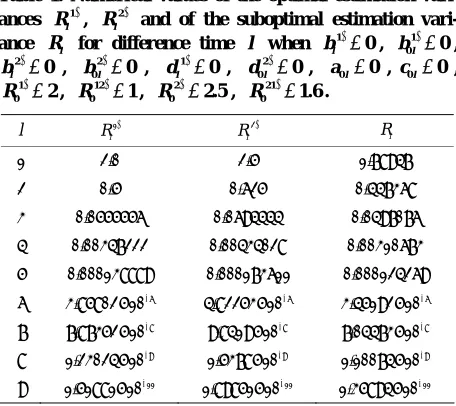
furthermore, substitute these into (52) and (53) then we can get , ; finally, substitute and into (55) then we can get . Numerical simulation re-sults are in Table 1.

 1

l

p p_l 2 p_l 1 p_l 2

[7] I. N. Sinitsyn, “Conditionally Optimal Filtering and Rec-ognition of Signals in Stochastic Differential System,”

Automation and Remote Control, Vol.58, No. 2, 1997, pp.

[image:5.595.58.286.516.719.2]

124-130.

Table 1. Numerical values of the optimal estimation vari-ances R l1 ,

 2

l

R and of the suboptimal estimation vari-ance R for difference time when l ,

[8] Y. Cho, V. I. Shin, M. Oh and Y. Lee, “Suboptimal Con-tinuous Filtering Based on the Decomposition of Obser-vation Vector,” Computers & Mathematics with Applica-tions, Vol. 32, No. 4, 1996, pp. 23-31.

doi:10.1016/0898-1221(96)00121-6

l bl 1 0

 1 0l 0

b  ,

, , , , ,

 2

l

b 0 b0 2l 0

 1

0

l

d  d0 2l 0 a0l 0 c0l 0,

, , , .

 1 0

R 2 R0 12 1  2 0

R 2.5 R0 21 1.6

l Rl 1

 2

l

R Rl [9] Y. Bar-Shalon and L. Campo, “The Effect of the

Com-mon Process Noise on the Two-Sensor Fused-Track Co-variance,” IEEE Transactions on Aerospace and Elec-tronic Systems, Vol. 22, No. 6, 1986, pp. 803-805.

doi:10.1109/TAES.1986.310815

1 2.0 2.5 1.78947

2 0.5 0.62

0.0694

0.004340 000173

4.82253

5 0.447368

3 0.0555556 444

28 611

6

10

0.0497076

4 0.00347222 0.00310673

5 0.000138889 0. 0.000124269

6 _{3.85802 10}_ 6 _ _{3.45192 10}_ 6

7 _{7.87352 10}_ 8

[10] I. N. Sinitsyn, N. K. Moshchuk and V. I. Shin, “Condi-tionally Optimal Filtering of Processes in Stochastic Dif-ferential Systems by Bayesian Criteria,” Doklady Mathe-matics, Vol. 47, No. 3, 1993, pp. 528-533.

[11] R. C. Luo and M. G. Kay, “Multisensor Integration and Fusion in Intelligent Systems,” IEEE Transactions on Systems, Man and Cybernetics, Vol. 19, No. 5, 1989, pp.

901-931.doi:10.1109/21.44007

8

10

9.8419 _{7.04473 10}_ 8

8 _{1.23024 10}_ 9 _1.5378_₁₀9 _{1.10074 10}_ 9

(6)

T. J. HE ET AL.

762

0 0

c

Appendix

Derivation of Formula (26). It follows from (16) that

         





   



   



   











   



   







   



   





1 1 1

2 1 1 2

2 0 0 2 0 0

2 0 0 2

1 2 1 δ δ δ δ δ δ δ

ij i j T

l l l

T

i i i jT j j

l l l l l l l l

T

i i T j j

l l l l l l l l

T n

i i T j j

l l l l l l rl rl lr

r i i

l rl rl r

R E X X

a b E X X a b

d c E V V d c

d c E V V d c X

d c                 _ _           _ _  _     



       





   











   



2 1 2 2 1 δ

δ δ ,

n

T lr l l

T n

j j T

lr l rl rl r

n T

i i T j j

l rl rl lr l l l l l r

X E V V

X d c

d c X E V V d c

   _{ } _         _  _     _  _   



(56)

set 0 ,

     

0 δ2 0

i i i

l l l

Q  d c_l Q_rl i ₂   i_ld_rli  _rl, then it fol-lows from (56) that

 



   



 



   



   

       

   

_

1 2 2 0

0 0

1 1

1

δ δ

; , 1, , .

T

ij i i ij i i i j T

l l l l l l l l l l l

n n

i jT i jT

lr l l rl lr rl l l

r r

n

i j T lrs rl l sl r

R a b R a a b Q G Q

m Q G Q m Q G Q

k Q G Q i j i j N

             







0l



l (57)

Derivation of Equation (27). We seek the optimal

ma-trices minimizing the mean square error, i.e.,

 i

_

_{1, ,} l

p i  N

 



     





     



1 , 1,

N N

i i iT i ij jT

l l l l l l

i i j i j

tr R tr p R p tr p R p

  









(58)

   

1 , 0.

N i i

l l

i p I p 



(59) Next, we use the following formulae





 

, , T T T

tr ABA AB AB

A

tr AB tr BA B

A A  _ _        (60)

to differentiate the function with respect to , we can derive that for any

 

l ,

tr R

 k l

p



k1, , N1



k

 



     



 



     



1 , 1, , N

i i i T

l l l l

k k

i

l l

N

i ij j T l l l k

i j i j l

tr R tr p R p

p p

tr p R p p     _ _{ }                _ _  _



substitute (59) into the following equation, we can derive that for any k,

 



     



           





        1 1 1 2 2 2

2 2 ,

N

i i i T l l l k

i l

k k N

l l l

N N N

l l l l

k k N N

l l l l

tr p R p p

p R R

p p p p

p R p R

                



 (62)  



     



 



     



 



     



 



     



, 1, 1 , 1, 1 1 1 1 , N

i ij j T l l l k

i j i j l

N

i ij j T l l l k

i j i j l

N

N Nj j T l l l k

j l

N

i iN N T l l l k

i l

tr p R p p

tr p R p p

tr p R p p                _ _     _ _        _ _        _ _   



(63)  



     



        1 , 1, 1 1 1, 1, . N

i ij j T l l l k

i j i j l

N N

j kjT i ik

l l l l

j j k i i k

tr p R p p

p R p R

                  



(64)

Substitute (59) into the following equations, we can derive that  



     



     





                  1 1 1

1 ( ) 1 1 1 1 1, 1, ( , N

i iN N T

l l l

k i l

N _N T

i iN j

l l j l

k i l

kNT k kNT k kNT

l l l l l

N N

j kNT i iNT

l l l l

j j k i i k

tr p R p p

tr p R I p

p

R p R p R

p R p R

   _                     _  _        



(65)  (61)  



     



 



 



                      1 1 1 1 1 1 1 1 1, 1, ( N

N Nj j T l l l k

j l

N

N j Nj j T

l l l

j k

i l

T

Nk k kN k Nk

l l l l l

N T N

j Nj i Nk

l l l l

j j k i i k

tr p R p p

tr I p R p

p

R p R p R

p R p R

   _                     _  _        _ _     _ _ 



(66)

for any k



k1, , N1



. Substitute (62)-(66) into 61), we can derive that

(7)

 

                       

 

   

 

     

1

1, 1

1,

1 1

2

N _T _T

j kj Nj k kk Nk

l l l l l l l

k

j j k l

N

i ik iN k kk kN

l l l l l l

i i k

N T N T T

j kN i kN kN Nk N

l l l l l l l l

j i

tr R p R R p R R

p

p R R p R R

p R p R R R p R



  

 

 

 

 _ _{ } _ _ _ _ _ _ _

  _ _ _ _



   

 _  _ _  _

    



 

       



   



       



   



1

1 1

1

,

NN

N T T

j kj Nj N kN N

l l l l l l

j

N

i ik iN N Nk N

l l l l l l

i

p R R p R R



 



 

 _  _  

 

 _  _ 



(67)