Survival, density, and abundance of common bottlenose dolphins in Barataria Bay (USA) following the Deepwater Horizon oil spill

INTRODUCTION

Photo-identification (photo-ID), the process of using photographs for individual recognition, has become a reliable, non-invasive technique for tracking small cetaceans temporally and spatially (Würsig & Jeffer-son 1990). The natural markings, principally nicks and notches along the trailing edge of common bottle

nose dolphin Tursiops truncatusdorsal fins, as well as body scars and pigmentation patterns, can persist throughout their lifetime (Lockyer & Morris 1990, Würsig & Jefferson 1990, Read et al. 2003). Capture-recapture analyses are commonly applied to photo-ID data to estimate abundance (Wilson et al. 1999, Read et al. 2003, Balmer et al. 2008) and survivorship (Speakman et al. 2010).

© The authors and (outside the USA) the US Government 2017. Open Access under Creative Commons by Attribution Licence. Use, distribution and reproduction are un restricted. Authors and original publication must be credited.

Publisher: Inter-Research · www.int-res.com *Corresponding author: tmcdonald@west-inc.com

Survival, density, and abundance of

common bottlenose dolphins in Barataria Bay (USA)

following the

Deepwater Horizon

oil spill

Trent L. McDonald

*, Fawn E. Hornsby

_{, Todd R. Speakman}

_{, Eric S. Zolman}

_,

Keith D. Mullin

, Carrie Sinclair

, Patricia E. Rosel

, Len Thomas

, Lori H. Schwacke

1_{Western EcoSystems Technology, Inc., Laramie, WY 82070, USA}

2_{National Centers for Coastal Ocean Science, National Oceanic and Atmospheric Administration, Hollings Marine Laboratory,} Charleston, SC 29412, USA

3_{National Marine Fisheries Service, Southeast Fisheries Science Center, Pascagoula, MS 39568, USA} 4_{National Marine Fisheries Service, Southeast Fisheries Science Center, Lafayette, LA 70506, USA}

5_{Centre for Research into Ecological and Environmental Modelling, University of St. Andrews, St. Andrews KY16 9LZ, UK}

ABSTRACT: To assess potential impacts of the Deepwater Horizon oil spill in April 2010, we conducted boat-based photo-identification surveys for common bottlenose dolphins Tursiops truncatusin Barataria Bay, Louisiana, USA (~230 km2_{, located 167 km WNW of the spill center).}

Crews logged 838 h of survey effort along pre-defined routes on 10 occasions between late June 2010 and early May 2014. We applied a previously unpublished spatial version of the robust design capture-recapture model to estimate survival and density. This model used photo locations to estimate density in the absence of study area boundaries and to separate mortality from permanent emigration. To estimate abundance, we applied density estimates to saltwater (salinity > ~8 ppt) areas of the bay where telemetry data suggested that dolphins reside. Annual dolphin survival varied between 0.80 and 0.85 (95% CIs varied from 0.77 to 0.90) over 3 yr following the Deepwater Horizonspill. In 2 non-oiled bays (in Florida and South Carolina), historic survival averages approximately 0.95. From June to November 2010, abundance increased from 1300 (95% CI ± ~130) to 3100 (95% CI ± ~400), then declined and remained between ~1600 and ~2400 individuals until spring 2013. In fall 2013 and spring 2014, abundance increased again to approx-imately 3100 individuals. Dolphin abundance prior to the spill was unknown, but we hypothesize that some dolphins moved out of the sampled area, probably northward into marshes, prior to initiation of our surveys in late June 2010, and later immigrated back into the sampled area.

KEY WORDS: Robust design · Photo-identification · Tursiops truncatus · Capture-recapture · Spatial-capture model

O

PEN

PEN

A

CCESS

CCESS

§Corrections were made after publication. For details see www.int-res. com/abstracts/esr/v33/c_p193-209/

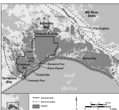
Currently, the National Marine Fisheries Service (NMFS) recognizes 31 Bay, Sound, and Estuary (BSE) stocks of common bottlenose dolphins in US waters of the northern Gulf of Mexico (GoM) (War-ing et al. 2015). The 31 stocks are treated as discrete populations because photo-ID and tagging studies, where conducted, generally provide evidence of long-term residency in BSEs of the northern GoM, and genetic studies have supported this concept (reviewed by Waring et al. 2015). Barataria Bay, Louisiana (Fig. 1), along with its ancillary bays (e.g. Caminada Bay and Bay des Ilettes) is located in the north-central GoM just west of the Mississippi River Delta, and comprises a single NMFS BSE stock (Waring et al. 2015). Few studies have estimated abundance and survivorship of common bottlenose dolphins in GoM stocks, including Barataria Bay

(Waring et al. 2015). One study, conducted between June 1999 and May 2002 (Miller 2003), identified 133 dolphins in the lower reaches of Caminada and Barataria Bays. This study produced an abundance estimate of 180 (95% CI 159 to 213), but only sam-pled a portion of Barataria Bay and thereby under-estimated the number of resident dolphins in the whole of Barataria Bay.

A catastrophic explosion on the Deepwater Horizon

(DWH) oil drilling rig on 20 April 2010 resulted in a fire that ultimately destroyed the rig 80 km ESE of the Mississippi River Delta (Port Eads, LA). The flow of oil from the uncapped well resulted in the worst marine oil spill in US history and released millions of barrels of crude oil into the northern GoM (DWH NRDA Trustees 2016). An unknown portion of the released oil ultimately penetrated the inshore waters

of Louisiana and Mississippi (DWH NRDA Trustees 2016), including Ba rataria Bay. In response, the National Oceanic and Atmo spheric Administration (NOAA) led a Natural Re source Damage Assessment (NRDA) to estimate damages to a wide variety of marine resources, in cluding the estuarine population of common bottlenose dolphins in Barataria Bay. NOAA researchers initiated boat-based photo-ID surveys in Barataria Bay in late June 2010. These sur-veys were designed to provide data on dolphin demographic parameters, specifically density, sur-vival, and abundance. Following capping of the DWH well in August 2010, photo-ID surveys contin-ued at sporadic intervals of 2 to 12 mo until April 2014, i.e. 4 yr after the spill began.

In this paper, we detail the photo-ID surveys in Barataria Bay, the photo processing necessary to identify individuals, and the subsequent statistical analysis of photo recaptures used to estimate survival and abundance. In doing so, we applied a previously unpublished variant of a spatially explicit capture-recapture model and made inference to changes in survival, density, and abundance during the 4 yr fol-lowing the spill.

FIELD AND PHOTO ANALYSIS METHODS Study area

The study area comprised estuarine waters of Barataria Bay near Grand Isle, Louisiana (29°14’ N, 90° 00’W), including Bayou Rigaud, Barataria Bay and Pass, Caminada Bay and Pass, Barataria Water-way, and Bay des Ilettes (Fig. 1). The study area is separated from the GoM by Grand Isle and the Grande Terre islands, but is connected by a series of passes to open GoM waters. The west, north, and northwest margins of the bay outside our study area include marsh, canals, channels, and bayous. The salinity of the bay’s water varies from nearly fresh northwest of the study area to nearly seawater in the south eastern tidally influenced portions sur-rounding the barrier islands (US EPA 1999, Moretz-sohn et al. 2010, and Hornsby et al. 2017, this Theme Section).

Photo-ID surveys

The field sampling methodology we employed has been standardized (reviewed by Rosel et al. 2011) and implemented by several studies in the

southeast-ern USA (e.g. Balmer et al. 2008, Speakman et al. 2010, Tyson et al. 2011). That methodology imple-ments a robust capture-recapture design (Pollock 1982, Kendall et al. 1995, 1997) containing secondary sampling occasions nested within primary sampling occasions. The robust design as sumes population closure among secondary occasions contained in the same primary, and openness between primaries.

Secondary occasions

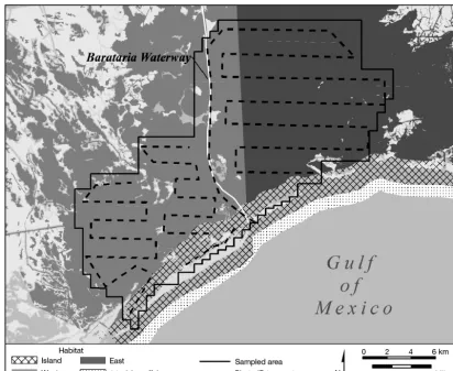
We defined a secondary sampling occasion to be 1 complete transit of our photo-ID transect (Fig. 2), which required approximately 2 d to complete and followed standard photo-ID field protocols (Melan-con et al. 2011, Rosel et al. 2011). We utilized two 5−6 m, center console, outboard vessels crewed by a minimum of 3 observers during all secondary sur-veys. On 1 day of a secondary survey, 1 vessel tar-geted Bara taria Pass’s southern half, while the other covered the pass’s northern half (Fig. 1). This was done to coordinate and adequately photograph the large number of dolphins typically encountered there. Outside Bara taria Pass, the 2 vessels operated independently and were nearly always out of line-of-sight.

We conducted most photo-ID surveys under opti-mal sighting conditions (Beaufort state < 3). Photo-ID vessels traversed the survey transect at 28− 30 km h−1_{until the crew sighted a dolphin or group}

of dolphins. We defined a dolphin group as all dolphins in relatively close proximity (<100 m), en -gaged in similar behavior, and generally heading in the same direction (Wells et al. 1980). After sighting a dolphin group, crews recorded the loca-tion of the boat after approaching within photo-graphic range. A handheld GPS device (Garmin GPSmap 76Cx, stated accuracy 10 m) onboard the boat determined all lo cations. One member of the crew attempted to photograph all members of a group, regardless of fin marks, using Canon EOS digital cameras equipped with 100–400 mm vari-able length telephoto lenses.

Primary occasions

We defined 3 consecutive secondary occasions, each separated by 1 d, to comprise a primary samp -ling occasion. The single day between secondary occasions was included to allow mixture of the dol-phin population. The 3 secondary occasions that made up each primary required approximately 1 wk to complete. We conducted 10 primary photoID oc -casions from late June 2010 through early May 2014 (dates listed in Table 1).

Photo analysis

Initial processing of photographs involved 4 gen-eral steps (Mazzoil et al. 2004, Melancon et al. 2011). Step 1 identified duplicate photos of individuals taken during a single sighting event. Step 2 selected the highest quality left- and right-side dorsal photo for each individual during each sighting event.

Often, only 1 side of an individual’s fin was pho-tographed during a sighting. Step 3 cropped each photo to isolate the dorsal fin. Finally, when neces-sary, we rotated the photograph to make the dorsal fin’s base parallel with the bottom of the frame. Occa-sionally, we adjusted brightness and contrast to improve image quality. We completed all processing in Photoshop 7.0 (Adobe Systems).

Correct identification of fins is critical to unbiased estimation of demographic parameters (Würsig & Jefferson 1990, Friday et al. 2000, Read et al. 2003). To help avoid false matches among photos, we graded the quality of images as Q-1 (excellent), Q-2 (average), or Q-3 (low) using a weighted scale based on 5 characteristics: focus, contrast, angle, fin visibil-ity/obscurity, and proportion of the frame filled by the fin (Urian et al. 2014).

We identified and matched individuals by visually comparing Q-1 and Q-2 photographs to other Q-1 and Q-2 photos in a catalog of dorsal fin photos. Photo graphs of lesser quality were occasionally

Fig. 2. Study area, showing common bottlenose dolphin Tursiops truncatusphoto-ID transects and habitat strata. The rectan-gular habitat mask used in analysis covered all shaded areas here and in Fig. 1, with land and ocean >2 km offshore coded

matched to known individuals if the fin was highly distinct and constituted a clear match. We stored and managed our dorsal fin photo catalog in a customized Microsoft Access database (FinBase) (Adams et al. 2006). Two researchers verified all matches, and hence all identifications. Following identification, we assigned unique numerical codes to the individual in FinBase. FinBase records also contained location, age class, distinctiveness, and other information pertain-ing to the fin or photo. We assigned distinctiveness based on the extent of dorsal fin markings, regardless of photographic quality. We considered fins with none or few markings to be ‘unmarked.’ We consid-ered very distinctive fins (coded D-1: obvious major marks) and average fins (coded D-2: 2 minor marks or 1 major mark) to be ‘marked’ (Urian et al. 2014). In each primary session, we estimated the proportion of marked dolphins in the population as the proportion of ‘marked’ fins among all high quality photographs (Q1 and Q2). Additional details of the photo ana -lysis are available in Melancon et al. (2011).

DATA ANALYSIS METHODS

We applied the spatially explicit robust design (SERD) model of Ergon & Gardner (2014) to dolphin photo-ID data from Barataria Bay after extending it to include habitat boundaries (wa ter). The SERD model of Ergon & Gardner (2014) incorporated a spatially

explicit capture− recapture (SECR) model (Borchers & Efford 2008) into the closed (within-primary) por-tion of a standard robust design and estimated den-sity, rather than abundance, for each primary occa-sion. SECR models estimate latent individual activity centers from the capture locations of every individual and use these locations to adjust capture probabili-ties based on distance to trapping locations. In turn, the distance-based capture probabilities estimate an ef fective study area, and density is essentially esti-mated as the number of activity centers divided by size of the effective study area. We extended the SERD model of Ergon & Gardner (2014) to include habitat boundaries (hereafter, ‘habitat mask’) that restricted dolphin movement and activity centers to water. The spatial capture heterogeneity induced by the SERD model allowed the open primary) portion to infer both permanent and tempo-rary emigration, thereby estimating ‘true’ rather than ‘apparent’ survival.

In the remainder of this section, we describe the SERD model and its estimation via Markov chain Monte Carlo (MCMC) sampling. Computer code to carry out estimation, written in the JAGS language (Plummer 2003), is provided in Supplement 2 at

www. int-res.com/articles/suppl/ n033p193_supp2. R. (with additional implementation details available in Supplement 1 at www. int-res. com/ articles/ suppl/ n033 p193 _ supp 1.pdf). We per formed analyses in JAGS version 4.0.0.

Session Date Island density West density East density Abundance

Est (95% CI) Est (95% CI) Est (95% CI) Est (95% CI)

1 26-Jun-10 8.2 (7.2, 9.2) 0.64 (0.61,0.68) 0.038 (0.028,0.061) 1303 (1164,1424) 2 12-Nov-10 11.3 (9.9,12.6) 0.95 (0.90,1.00) 0.726 (0.532,1.155) 2270 (1960,2612) 3 9-Apr-11 11.8 (10.4,13.2) 1.20 (1.14,1.26) 0.270 (0.197,0.429) 2115 (1877,2290) 4 12-Jun-11 17.0 (14.9,19.1) 1.18 (1.12,1.24) 0.757 (0.555,1.204) 3107 (2700,3485) 5 14-Nov-11 10.0 (8.8,11.2) 1.61 (1.53,1.69) 0.625 (0.458,0.994) 2278 (1998,2576) 6 14-Feb-12 6.8 (5.9, 7.6) 1.14 (1.09,1.20) 0.674 (0.494,1.072) 1730 (1496,2030) 7 15-Apr-12 10.8 (9.5,12.1) 1.04 (1.00,1.10) 0.971 (0.711,1.544) 2412 (2064,2847) 8 12-Apr-13 10.2 (8.9,11.4) 0.69 (0.65,0.72) 0.113 (0.083,0.179) 1618 (1435,1759) 9 13-Nov-13 13.6 (11.9,15.2) 1.88 (1.79,1.98) 0.991 (0.726,1.577) 3078 (2673,3537) 10 27-Apr-14 14.3 (12.5,16.0) 2.11 (2.01,2.22) 0.850 (0.622,1.351) 3150 (2759,3559) Average density 11.4 (9.99,12.8) 1.24 (1.19,1.31) 0.601 (0.441,0.957)

SD(density) 0.884 0.0319 0.185

Average abundance 1452 (1272,1625) 442 (421,465) 412 (302,655) 2306 (2014,2603)

SD(abundance) 112.6 11.3 126.6 195.9

Table 1. Estimated posterior mean common bottlenose dolphin Tursiops truncatusdensity (ind. km−2_{) and abundance (no.} dol-phins) during primary capture sessions, and averaged over the study period in Barataria Bay, Louisiana (USA). CI: lower and upper credible interval. All values are plotted in Fig. 6. Abundances were calculated by expanding densities to the size of the stratum. Sizes of the strata were: 127.379, 355.278, and 684.728 km2_{for Island, West, and East, respectively. Stratum densities}

Spatially explicit component for density

The SECR (i.e. closed) component of our SERD mo del mimicked that of previous SECR models (Bor -chers & Efford 2008, Royle et al. 2013, Schaub & Royle 2014). We divided the sampled area (Fig. 2) into a total of R square discrete pixels, each with size

1000 × 1000 m. These pixels were considered traps, and an individual became caught in a trap when its photo location plotted inside the pixel boundaries. Below, we use the term trap rather than pixel for gen-erality, but in this study trap and pixel are synony-mous. During a particular secondary sampling occa-sion, an individual could be caught in at most one trap, but one trap could capture multiple individuals during a secondary occasion. Individual capture his-tories for a primary session consisted of at most 3 trap identifiers, one for each secondary occasion. When an individual was not photographed, the trap identi-fier did not exist. For computational reasons that will become apparent later, the trap identifier for known un-captured individuals was set to 0.

Data and notation

The number of subscripts required to fully specify the model is excessive. In the following, we generally adopt the notation of Ergon & Gardner (2014), but use arrays for clarity and to make implementation straightforward. To reference an element of an array, we use brackets (i.e. [ ]) instead of subscripts. For example, when g is a parameter, we write g[i,k,t]

instead of gikt. When Gis an array, we write G[i,j,k] to

reference the ithrow, jthcolumn, and kthpage. When

we omit a dimension from the brackets, we reference the entire missing dimension, which is generally a vector. For example, G[i,,k] references all columns

from the ithrow and kthpage of G. This latter

nota-tion is modeled after R language syntax (R Core Team 2015) for referencing multi-dimensional arrays. One-dimensional arrays are vectors. Two-dimensional arrays are matrices. Vectors, matrices, and arrays are in boldfont, scalars are in italicfont.

We start by defining npto be the number of

pri-mary occasions, and nsto be a vector of length np

containing the number of secondary occasions in each primary. Here, ns=[3,3,…,3]. We define nto be

the number of unique individuals captured during all primary and secondary occasions. We define nsmaxto

be the maximum number of secondary occasions that occurred during a single primary (i.e. nsmax =

max(ns); here, nsmax= 3). Let dt be an np−1vector

of time intervals (fractions of a year) between each primary.

Trap locations are housed in matrix X, which is size

R× 2. X[r,] is the (x,y) coordinate vector of the center

of trap r. Capture histories in the form of trap indices

are housed in a 3-dimensional array Hwhich has size

n× nsmax× np.H[i,j,k] is the row index of Xfor the

trap that captured individual i during secondary

occasion jof primary session k. In other words, the

trap at location X[H[i,j,k],] captured animal iduring

secondary j of primary k. Prior to first capture and

when a previously captured animal was not cap-tured, H[i,j,k] = 0; but values prior to first capture

were inconsequential because the model conditions on first capture. For computational purposes X[0,]

was understood to be the null, or nonexistent, location.

In regular SECR models (e.g. Borchers & Efford 2008, Ergon & Gardner 2014, Schaub & Royle 2014), individuals are viewed as having a single activity center during the study period. Activity centers are latent, or unobserved, in SECR models because loca-tions are only known when an individual is seen. Here, we allow different activity centers on each primary occasion. For computational purposes, we de -fine array Sto be an n× 2 × nparray such that S[i,,k]

is the (x,y) coordinate vector of individual i’s activity

center during primary session k.

We incorporated a habitat mask into the SERD model by defining Mto be an mx× mymatrix of 0’s

and 1’s, where each cell was associated with a geo-graphic pixel (1000 × 1000 m). Cells in Mcontaining

1’s indicated pixels where activity centers could be located, while 0’s indicated pixels where activity cen-ters could not be located. We set the size of Msuch

that it covered a large area surrounding the sampled area (lower-left inset, Fig. 1). Values asso ciated with pixels whose centers fell on land or were over 2 km offshore of the islands were set to 0. We set values in

Mto 1 when a pixel’s center fell in water and within

2 km offshore of an island. For computational con-venience, we set the origin of the mask so that habi-tat pixel centers coincided with trap pixel centers in the sampled area, but this was theoretically not nec-essary. To facilitate programming via simple index-ing and to simplify specification of priors, we shifted the locations in X, M, and Z(Zdefined in next

para-graph) left and down so that the minimum horizontal and vertical coordinate was (0,0).

hypothesized that density varied among 3 habitat areas (i.e. strata). The ‘Island’ stratum encompassed waters less than 1 km from 1 of the barrier islands (Fig. 2). The ‘West’ stratum primarily encompassed non-island portions of Barataria Bay west of the Barataria Waterway (Fig. 2). The ‘East’ stratum en -compassed non-island portions of the bay east of the waterway. Due to the shape and slight curvature of islands in the Island stratum, it was possible for a dol-phin’s activity center to fall outside the Island stratum (>1 km from islands) even though dolphins were only photo graphed inside the Island stratum. To allow this situation, we included a fourth stratum defined as waters between 1 and 2 km offshore of the barrier islands, but we do not report density estimates there because we inadequately sampled dolphins in this area. The stratum designation of all pixels in non-habitat (M= 0 pixels) was unassigned because they

were not used in calculations. The end result was an

mx× mymatrix Z, similar to M, of strata indicators 1,

2, …, 5 with 1 = Island, 2 = West, 3 = East, 4 = 1−2 km offshore, and 5 = non-habitat.

Capture probability model

As in standard SECR models, we modeled the cap-ture probability of an individual as a function of dis-tance between its activity center and all traps. We used the exponential power series capture function (Pollock 1978) to model the decline in capture prob -ability of activity centers far from the traps. During a particular primary occasion, we modeled the expo-sure of an individual with activity center at S[i,,k] to

our photographic efforts in trap X[t,] as

(1)

where d[i, k, t] = ((S[i, 1, k] − X[t, 1])2+ (S[i, 2, k] −

X[t, 2])2)0.5 was distance (in units of pixels, here km)

between the activity center and the trap. Parameters

λm, σm, and κm (m = 1, 2, 3, 4) were strata-specific

parameters that determined the height, extent, and shape of the capture function (Fig. 3).

The prior distributions for σm and κm were: σm ~

Uniform(0.1, 15); κm~ Uniform(1, 3) for m= 1, 2, 3, 4.

The prior for σm was considered uninformative be

-cause, at the upper limit of 15, substantial capture hazard existed at every trap for individuals in almost all parts of the sampled area. Note that the upper limit of 15 km was approximately the entire north− south extent of the study area (Fig. 2) and half of the east−west extent of the study area. Many authors do

not estimate κm and simply assume the half-normal

capture function (i.e. κm= 2) (Borchers & Efford 2008,

Schaub & Royle 2014), so we chose a mildly informa-tive prior distribution for κmcentered on 2.

The capture function intercept, λm, quantified the

probability of detection at a single trap assuming that an activity center coincided with the trap location. The prior distribution for λmdepends upon the

num-ber and configuration of traps, as well as the size of an individual’s activity area. We did not have a prior estimate of λmand consequently specified a uniform

prior as λm ~ Uniform(0.002, 0.02). This prior for λm

covers the approximate range of the number of traps in a dolphin’s presumed activity area. Based on radio telemetry, we estimated a dolphin’s activity area dur-ing a primary session to contain between 1 and 10 traps, and set the limits of λm’s prior to approximately

1/Rand 10/R(where R= number of traps).

The overall exposure of individual i to trapping

during any secondary occasion in primary kwas

G[i,k] =

Σ

t=1g[i,k,t] (2)

The overall probability of capturing a photograph of individual i’s dorsal fin in any trap during any of

the secondary occasions of primary occasion kwas

p[i,j,k] = 1 − exp(−G[i,k]) (3)

Here, G[i,k] does not contain an index for

second-ary occasion (i.e.j) and therefore does not vary by se

condary occasion. Models which vary capture prob -ability over secondary occasions are possible, but

[ , , ] exp – [ , , ]

g i k t m d i k t m

m

= λ

σ ⎛

⎝⎜ ⎞⎠⎟

⎛ ⎝⎜

⎞ ⎠⎟ κ

Fig. 3. Plots of capture exponential power series functions for an individual trap (Eq. 1) for 3 hypothetical values of shape parameter κ, height parameter λ= 0.006, and extent

were not needed here given the extremely short du -ration of primary sessions (~1 wk).

The probability of capturing a photograph of indi-vidual iin trap tduring secondary occasion j of

pri-mary session kwas modeled as

(4)

and the probability of not photographing the indivi -dual was

Pr(H[i,j,k] = 0) = 1 − p[i,j,k] (5)

Derived density estimates

Given a sample of the capture parameters [λm, σm,

κm] from their posterior distribution, we derived

esti-mates of density after Borchers & Efford (2008). In this section, the number of indices is excessive if we maintain one for the primary occasion (i.e. kabove).

Consequently, we drop the index for primary occa-sions and conduct the following calculations for each primary.

Conceptually, we derived a density estimate in themth stratum by hypothesizing activity centers in

every pixel of valid habitat and computing probabil-ity of detection in every pixel. We then estimated density as the observed number of captures divided by the sum of all activity center capture probabilities in valid habitat.

Assume the number of valid habitat locations in M

is q(i.e. q= number of 1’s in M=

Σ

i=1

Σ

Cbe a q× 2 matrix containing the (x,y) coordinates

for the centers of all valid habitat pixels in M. Given

an estimated parameter vector [λa

m, σam, κam] from the

MCMC routine (aindicates the athMCMC iteration),

we evaluated the capture function (Eq. 1) as

(6)

where d[i, t] = ((C[i, 1] − X[t, 1])2 + (C[i, 2] −

X[t, 2])2)0.5is the distance from location C[i,] to trap t.

We computed overall exposure of an activity center at C[i,] to capture as

G[i,a,m] =

Σ

t=1g[i,a,m,t] (7)

and the probability of obtaining a photograph of an animal with activity center C[i,] during a single

sec-ondary occasion as

p[i,a,m] = 1 − exp(−G[i,a,m]) (8)

Because we modeled constant capture probabili-ties across secondary occasions, the probability of

photographing an individual during ns[k] secondary

occasions was

P[i,a,m] = 1 − (1 −p[i,a,m])ns[k] ₍₉₎

Here,P[i,a,m] was equivalent to ‘p.(x)’ of Borchers

& Efford (2008). For each iteration awe summed the P[i,a,m] surface over all habitat locations ito arrive at

a probability of detecting individuals in stratum mon

iteration a, i.e.

A[a,m] =

Σ

i=1P[i,a,m] (10)

Finally, we defined the number of individuals pho-tographed in stratum mduring the primary occasion

to be n[m] and computed density as

(11)

where b is the proportion of distinctive fins seen

during the primary session. We computed bas the

fraction of all high quality photographs with enough distinctive marks to uniquely identify the individual. Inclusion of binflated density estimates to account

for the unmarked population fraction, which typi-cally represented young individuals. Our model did not include variation in the estimated b because

the proportion was relatively high (approximately 0.8) and based on hundreds of photos (conse-quently, se(b) = is small). The point

estimate of density in stratum m was the posterior

mean, obtained by computing average D over the

MCMC iterations (i.e. over a) after a suitable

burn-in period (see below). A 95% posterior credible interval (CI) for density was computed by calculat-ing the 2.5th_{and 97.5}th_{quantiles of D[a,m] over all}

MCMC iterations.

Derived abundance estimates

We estimated abundance by expanding specific density estimates to the area of estimated dolphin habitat in Barataria Bay. Estimated dolphin habitat was derived by Hornsby et al. (2017), who used daily salinity maps and daily dolphin satellite-tag-telemetry locations to estimate an average mini-mum salinity level tolerated by dolphins. Hornsby et al. (2017) estimated that 95% of dolphin locations occurred in waters more saline than 7.89 ppt. By averaging the daily location of the 7.89 ppt salinity contour over multiple years, Hornsby et al. (2017) estimated 1167.385 km2 _{of dolphin habitat in Bara}

-taria Bay (grey areas in Fig. 1) apportioned among the strata as follows: Island habitat = 127.379 km2_;

[ , , , ] exp [ , ]

g i a m t ma d i t m a

m a

=λ − σ ⎛ ⎝⎜ ⎞⎠⎟ ⎛

⎝⎜

⎞ ⎠⎟ κ

n

[ , ] [ ]

[ , ] 1

D a m m

A a m b

=⎡

⎣⎢

⎤ ⎦⎥

(1 ) /

b −b n

H

Pr( [ , , ] ) [ , , ]

[ , ] [ , , ],

i j k t g i k t

G i k p i j k

West habitat = 355.278 km2_{; and East habitat =}

684.728 km2_.

Reinstating the subscript for primary session (i.e.

k), we computed an estimate of abundance from every

iteration of the MCMC routine as

N[k,a] =

Σ

where K [m]is total area of stratum m (in km2) and D[k,a,m]is density estimated for the kthprimary on

the athiteration of the MCMC sampler in stratum m.

The final point estimate of abundance for the primary session was the mean N [k,a]over MCMC iterations.

We computed lower and upper CI limits as the 2.5th_and

97.5th_{quantiles of the mean over MCMC iterations.}

To arrive at a single estimate for the entire study period, we averaged Nover the npprimary occasions

each MCMC iteration. Lower and upper CI limits were the 2.5th_{and 97.5}th_{quantiles of this average.}

Open component for survival

The SERD model allowed population changes and activity center movements between primary sions. We estimated survival between primary occa-sions following Ergon & Gardner (2014) who condi-tioned on first capture and followed individuals afterwards, similar to Cormack-Jolly-Seber models (Jolly 1965, Seber 1965, Cormack 1972, Schaub & Royle 2014).

Movement model for activity centers

We assumed the activity center associated with an individual’s first primary had a (bivariate) uniform prior over the habitat mask. We assumed

S[i, ,f ]~Uniform([0, Δx], [0, Δy]) (13)

where Δx is the horizontal extent of our habitat

mask, Δyis the vertical extent of our habitat mask,

and fis the first primary during which we

encoun-tered animal i. Here, Δx= mxkm and Δy= mykm

because we used 1 km grid cell spacing. During MCMC sampling, we employed the habitat check of Meredith (2013) to assign probability 0 to S[i, ,f] if

M[sx, sy] = 0, where sx = floor(S[i,1,f]) and sy = floor(S[i, 2,f]) and floor(x)is the largest integer less

than or equal to x. This prevented placement of

activity centers in pixels with M= 0. Had we used a

grid spacing other than 1 km, we would have divided S[i,1,f] and S[i,2,f] by their respective cell

extents prior to applying floor.

Following first encounter, a simple movement mo del based on distance and angle allowed different ac -tivity center locations during each primary occasion (Schaub & Royle 2014). We computed a new activity center location for primary occasion k> fas

S[i,1,k] = S[i,1,k − 1] + d[i,k − 1]cos(θ[i,k−1]) (14)

S[i,2,k] = S[i,2,k − 1] + d[i,k − 1]sin(θ[i,k−1]) (15)

where θ[i,k−1] ~ Uniform(−π, π), d[i,k – 1]~ Expo-nential(γm–1) and γm(m= 1, …, 5) was a

stratum-spe-cific hyper-parameter for movement distance. The prior for γmin stratum m= 1, 2, 3, or 4 was uniform

on the interval [0,20], while γ5was fixed at an

arbi-trary value (0.5) because activity centers were not allowed outside the habitat mask where stratum was ‘non-habitat.’ Again, a habitat check ensured that activity centers in non-habitat were assigned zero prob ability.

Conditional likelihood for survival

To aid interpretation and facilitate later summaries, we parameterized the open portion of the SERD model using equivalent annual survival, which we assumed had a uniform(0,1) prior distribution. We

adjusted for unequal time intervals between primar-ies by defining w[k] (k= 1, 2, … (np− 1)) to be the

fraction of a year between primary occasion k and k+1 and raising the equivalent annual survival, Φ[k]

(k= 1, 2, … (np−1)), to the w[k] power. For example,

if 6 mo elapsed between primary occasions 1 and 2, while 15 mo elapsed between occasions 2 and 3, w=

[0.5, 1.25] and the interval-specific survivals were

Φ[1]0.5_{and Φ[2]}1.25_.

More specifically, let z[i,k] be a n × npmatrix of

latent (unobserved) 0’s and 1’s where z[i,k] = 1 if

individual iwas alive during primary k, and 0

other-wise. Note that z[i,f]= 1 always, z[i,k+1] = 0 if z[i,k]=

0, and z[i,k]for k< fwere inconsequential be cause

they did not enter the conditional likelihood. Given latent survival indicator z[i,k], the likelihood of

ani-mal isurviving to primary session k+1 was

Pr(z[i,k+ 1] = 1) = z[i,k]Φ[k]w[k] ₍₁₆₎

approximately 1 yr in length. We therefore summarized survival during 4 combined inter-vals (each starting and ending at a primary session, Table 2) by averaging the equivalent annual survival estimates over the between-primary periods in each. For example, the sec-ond combined interval following the spill started on 12 June 2011 and lasted until 15 April 2012, a period of 10 mo. This period con-tained 3 inter-primary intervals and hence 3 estimates of the equivalent annual survival (i.e. Φ[4], Φ[5], and Φ[6]). We estimated proba-bility of surviving the second combined inter-val as

(17)

We performed similar calculations for the other 3 combined intervals listed in Table 2, as well as aver-aged equivalent annual survivals over the same intervals.

MCMC estimation

We implemented 3 parallel MCMC chains in JAGS to estimate parameters. Each chain per-formed 500 burn-in steps and 200 sampling steps. Iterations took approximately 9 d to complete on a single-core 64-bit server, and ultimately yielded 600 observations of the parameter vector. The Gel-man and Rubin procedure (GelGel-man & Rubin 1992) checked mixing of the λm, σm, κm, and Φchains by

computing potential scale re duction factors. Geweke

z statistics checked convergence of the

chains (Geweke 1991).

RESULTS

Crews photographed 1601 unique indi-vidual common bottlenose dolphins dur-ing 10 primary occasions in Bara ta ria Bay. Intervals between primary oc casions var-ied from 2 mo to 1 yr. The number of unique individuals per primary varied from 226 (Primary 1) to 591 (Primary 10) (Fig. 4). The cumulative number of new individuals (i.e. the discovery curve) lev-eled off between April 2012 and April 2013, but then continued to grow during late 2013 and 2014 at a rate only slightly lower than previously observed (Fig. 4).

Mixing of all parameters, especially survival para -meters (Φ[k], k = 1,…,9), was good, except for capture

parameters σ1and κ1associated with the Island

stra-tum (with potential scale reduction factors of 4.9 and 5.7, respectively), and σ3 and λ3 associated with the

East stratum (potential scale reduction factors 10.8 and 4.2, re spectively). The Geweke statistics in dicated convergence of all parameters except κ1 as sociated

with the Island stratum (z= 2.08), and σ3and λ3

asso-ciated with the East stratum (z = 9.01 and 2.22,

re-spectively). The estimated posterior mean σ1 was

2.34 km (95% CI = 2.18 to 2.52 km), while mean κ1

was 2.73 (95% CI = 2.17 to 2.99). The posterior mean of σ3 equaled 11.3 km (95% CI = 5.3 to 15.0 km),

while mean λ3 was 0.00229 (95% CI = 0.00200 to

0.00353).

It is not surprising that detection parameters con-verged slowly. All 3 parameters (λ, σ, κ) are corre-lated, and the detection function (Eq. 1) was nearly horizontal (its theoretical up per limit) in the Island

*[2] [4] [5] [6]

3

10/12 Φ =⎛_⎝Φ +Φ +Φ ⎞_⎠

Fig. 4. Discovery curve (cumulative number of unique individuals) and the number of individual common bottlenose dolphins Tursiops trunca-tuscaught per primary session. Tick marks on the x-axis are mid-point

dates of the primary sessions (listed in Table 1) Inter- Start End Interval Annual val Est. Low High Est. Low High

1 Jun 10 Jun 11 0.846 0.787 0.901 0.862 0.808 0.916 2 Jun 11 Apr 12 0.827 0.790 0.862 0.792 0.738 0.839 3 Apr 12 Apr 13 0.804 0.766 0.847 0.803 0.764 0.846 4 Apr 13 Apr 14 0.973 0.937 0.996 0.973 0.934 0.996 Table 2. Estimated common bottlenose dolphin Tursiops truncatus survival probabilities (‘Est.’) and 95% credible intervals (‘Low’, ‘High’) in Barataria Bay. ‘Interval’ estimates are probability of sur-viving the specific interval, computed by Eq. 17. ‘Annual’ estimates are the equivalent annualized survival computed by averaging

and East strata. Nearly constant detection out to 2+ km in the Island stratum was not surprising given the size of the strata, the ubiquity of dolphins in these areas, and the relative ease of spotting dolphins in waters around the islands. A low and attenuated (long) detection function in the East stratum was not surprising given its low density and predominantly open water habitat.

Survival

Across the first 3 combined intervals (approximately 3 yr following the DWH spill), estimated annual sur-vival of dolphins in Barataria Bay varied from 0.80 to 0.85, with upper credible limits at or below 0.90 (Table 2, Fig. 5). During the fourth and final 1 yr interval, we estimated survival to be 0.97 (95% CI = 0.94 to 0.99). The final interval includes survival be -tween the last 2 occasions, which is generally consid-ered unreliable in capture-recapture analyses due to partial or complete confounding with capture prob -ability (Lebreton et al. 1992).

Density

Estimated density (ind. km−2_{) of dolphins in the Is}

-land stratum was approximately 10 times higher than density in the 2 non-Island strata. Estimated density in the Island stratum increased from approximately 8.2 ind. km−2 _{in late June and early July 2010 to}

approximately 17.0 in June 2011 (Fig. 6). After June 2011, estimated density surrounding the islands varied from 6.7 to 10.8 ind. km−2 _{until November}

2013. After November 2013, density increased to 13.60 and 14.25 ind. km−2 _{in late 2013 and spring, 2014,}

respectively.

Density in the 2 non-Island strata remained rela-tively constant until November 2013. In the West stratum, density varied from 0.64 to 1.6 ind. km−2

until the April 2013 session when density during the final 2 primaries increased to 1.87 and 2.11 ind. km−2_.

In the East stratum, density varied between 0.03 and 0.97 ind. km−2_{until April 2013. Afterwards, density in}

the East stratum increased to 0.99 in November 2013 and 0.85 ind. km−2_{in April 2014.}

Abundance

Temporal trends in abundance mirrored temporal trends in density. In the year following the DWH spill, the estimated number of dolphins within Barataria Bay increased from 1300 (95% CI ± ~130) to 3100 (95% CI ± ~400) (Table 1, Fig. 6). Between summer and late fall 2011, the number of dolphins in Bara -taria Bay declined to approximately 2300 (95% CI ± ~290) individuals, and remained between ~1600 and ~2400 individuals until spring 2013 (Table 1, Fig. 6). In fall 2013 and spring 2014, the estimated number of dolphins in Barataria Bay increased to higher levels of approximately 3100 individuals (Table 1, Fig. 6).

DISCUSSION

Estimated survival rates for dolphins in Barataria Bay during the first 3 yr (2011−2013) after the April 2010 DWH oil spill were low (range 0.804− 0.846, Table 2) relative to other BSE common bottlenose dolphin stocks along the southeast US coast that have been studied with similar mark-recapture techniques. An an nual survival rate of 0.951 (95% CI = 0.88− 1.00) was re -ported for the Charleston BSE common bottlenose dolphin stock surveyed be -tween 2004 and 2006 (Speakman et al. 2010). Similarly, an annual survival rate of 0.962 was reported for common bottlenose dolphins in Sarasota Bay, Florida, surveyed over a 7 yr period

from 1980 to 1987 (Wells & Scott 1990). However, it was not surprising that we found lower survival rates in Barataria Bay dolphins given that an unusual mor-tality event (UME) in the northern GoM overlapped our study period (Litz et al. 2014, Venn-Watson et al. 2015). A UME as defined under the Marine Mammal Protection Act (116 USC 1421h) can be declared based on a number of criteria. In this case, the strand-ing rate was determined to be unusually high (over 2 SD above the historic mean rate). While the UME was declared for the broader northern GoM (Frank lin County, FL, to the Louisiana− Texas border), dolphin strandings were particularly high in Barataria Bay. In fact, Louisiana recorded the highest stranding rates on record between the April 2010 DWH spill and De-cember 2011 (Venn-Watson et al. 2015), and a large portion of these strandings were recovered in and around Barataria Bay. The number of dolphin strand-ings decreased in 2014 and the UME officially ended in July 2014. NOAA concluded that the DWH oil spill was the most likely explanation for the eleva ted stranding numbers that persisted for the 4 yr after the

spill (www. nmfs. noaa. gov/ pr/ health/ mmume/ cetacean _ gulf ofmexico.htm). Near the end of the UME period, our final survival estimate (April 2013 − April 2014) re bounded to 0.973 (95% CI: 0.937− 0.996) and was similar to rates re ported in previous studies of BSE dolphins (Wells & Scott 1990, Speakman et al. 2010). Despite our caution about confoun ding in the final survival estimate, the magnitude of the estimate makes it likely that sur-vival increased during the fourth 1 yr study interval relative to previous in-tervals, and this increased survival in late 2013 is consistent with lower dol-phin stranding numbers reported after April 2013 (relative to previous years). The density of common bottlenose dolphins varied spatially across the photo-ID survey area, with nearly 10-fold higher density observed in the Is-land stratum as compared to the 2 non-Island strata (Fig. 6). It is known that interlinked physical and biological fac-tors can cause increased density of top predators in specific areas (e.g. Wing-field et al. 2011). The multiple passes and estuarine entrances within the Is-land stratum (Fig. 1) likely provide at-tractive habitat for bottlenose dolphins. The entrances tend to concentrate fish moving be-tween estuary and ocean waters (Shane 1990) and must be negotiated by spawning fish when they move from medium to higher salinity waters in the GoM (e.g. Lyczkowski-Shultz et al. 1990). Addition-ally, sloping bottom topo graphy around islands can increase fish concentrations and facilitate dolphin foraging (Ingram & Rogan 2002). The higher density of dolphins observed in the Island stratum is also consistent with numerous prior studies in the GoM (Shane 1977, Barham et al. 1979, Leather wood & Reeves 1983) and elsewhere (Ballance 1992, Ingram & Rogan 2002) that indicate a tendency of bottlenose dolphins to aggregate near the entrances to estuaries. The densities estimated for the 3 strata, as well as the estimated overall abundance for the Barataria Bay stock, also varied temporally (Table 1, Fig. 5). Low densities for all 3 strata were observed in the first sampling occasion immediately following the DWH spill (June 2010). Densities increased over the following year, but then declined to varying degrees between June 2011 and April 2013. In the final 2

Fig. 6. Overall estimated (a) abundance and (b,c) density estimates of com-mon bottlenose dolphins Tursiops truncatusby stratum in Barataria Bay from the spatially explicit, robust design capture-recapture model. Points are esti-mated posterior means and vertical bars are 95% credible intervals. Symbols are plotted at the mid-point dates of primary sampling sessions. Dashed horizontal lines are temporal averages of their respective time series. Note

surveys (November 2013 and April 2014) densities across all 3 strata again increased and a concomitant uptick appeared in the discovery curve after a previ-ous apparent leveling off (Fig. 4).

NRDA photoID surveys did not begin until ap -proximately 2 mo after the DWH spill. Consequently, common bottlenose dolphin abundance in Barataria Bay prior to the DWH spill is unknown. By the time of the first photo-ID survey, oil response and cleanup activities were well underway. The heaviest and most persistent shoreline oiling occurred in portions of Barataria Bay (Michel et al. 2013), and thus this area immediately became a primary focus for oil spill response and the media. Hundreds of vessels respon -ded to oil in the nearshore environment, and activi-ties in the Barataria Bay area included placing and moving oilretention booms, skimming, dredging ac -tivities offshore of the islands, transport of response workers, officials, and journalists, and releases of fresh water from the Mississippi River. Over 12.7 mil-lion feet of oil containment boom was deployed in the northern GoM, including in Bara taria Bay, and both the boom deployment and sub sequent deployment of boom removal teams significantly increased boat traffic (DWH NRDA Trustees 2016). The unprece-dented level of boat activity and boom de ployment damaged nearshore habitats and disturbed wildlife (DWH NRDA Trustees 2016). Much of these cleanup activities overlapped photo-ID survey routes, partic-ularly the Island stratum. In addition, fishing and shrimping activities were temporarily banned in parts of the bay. While the spatial and temporal clo-sures of fishing activity during 2010 were extremely complicated and not well documented, the general reduction in fishing would have reduced bycatch that is likely an attractive food source to some dolphins. We suggest that the combined effects of response, cleanup, preventative activities, and reduced fishing, as well as the oil itself, created an unfavorable envi-ronment for dolphins throughout much of Barataria Bay. Faced with this unfavorable environment, it is very plausible that dolphins responded by temporar-ily moving out of areas near barrier islands and passes where the most intense cleanup activities were oc -curring (Fig. 7a). Dolphins that may have moved to marshes in the extreme interior (north, west, or east) would not have been photographed.

While not comparable to the unprecedented level of disturbance in Barataria Bay, prior studies have also observed temporary shifts in distribution related to disturbance by industrial activities. A change in bottlenose dolphin density was observed in Sarasota Bay during bridge construction, with dolphin density

increasing in the vicinity of the bridge once construc-tion was complete (Buckstaff et al. 2013). A study of bottlenose dolphins in Aberdeen Harbor, Scotland, found that dredging operations temporarily displaced bottlenose dolphins from an important for -aging area (Pirotta et al. 2013). Similarly, harbor por-poise density decreased in the vicinity of an offshore wind farm during construction that involved driving activity (Dähne et al. 2013).

Estimated abundance increased during surveys after the well was capped, when spill-related anthro-pogenic activities slowed (November 2010 to June 2011) and eventually ceased. At that time, it is possi-ble that the reduced activity level prompted dis-placed dolphins to return to portions of the bay sub-ject to our photo-ID efforts (Fig. 7b).

The decline in densities across the 3 strata after June 2011 and continuing until April 2013 is consis-tent with a population experiencing increased mor-tality (Fig. 7c). Our low survival estimates for this period, concurrent high stranding rates, and general poor health of Barataria Bay dolphins documented during separate health assessments (Lane et al. 2015, Smith et al. 2017, this Theme Section) strongly sup-port the notion that increased mortality occurred dur-ing this period.

Mississippi Sound was a response to greater resource availability caused by decreased fishery activities after Hurricane Katrina 2 yr earlier. If a similar in -crease in dolphin reproduction occurred in Barataria Bay during the same time period, the larger-than-normal calf cohort would have been 6 to 7 yr old at the time of the final 2 photo-ID surveys.

However, despite the possibility that a large num-ber of dolphins became distinctive in mid-2013, we believe that increased reproduction alone cannot ex -plain the nearly 50% increase in density for the Island stratum, and the 3fold and nearly 8fold in -crease in density for the West and East strata, respec-tively, in a 1 yr period (April 2013 to April 2014). Even a significant increase in calving over a 2 to 3 yr period (e.g. beginning in 2007 concurrent with the calving boom reported for Mississippi Sound, and continuing until 2010 when the DWH oil spill oc -curred) would not be sufficient to produce such large proportional increases in densities. Such increases

translate into nearly doubling the estimated overall dolphin abundance, over a very short period.

Instead, we suggest that the apparent influx of new dolphins likely represents movement of distinctive individuals from peripheral habitat, within Barataria Bay but outside the photo-ID study area, into the photo-ID study area where they would be subject to our photographic efforts (Fig. 7d). The loss of dol-phins through mortality over the prior 2 yr period would have created space and potentially freed other resources. The freeing of resources then could have prompted the movement of other dolphins into the photo-ID study area from more peripheral habitat, such as the more variable and generally lower salin-ity waters to the northwest. An analysis of telemetry data from Barataria Bay bottlenose dolphins inte-grated with a spatio-temporal model of salinity pat-terns, indicated that the tagged dolphins favored higher salinity waters (DWH MMIQT 2015, Hornsby et al. 2017). Furthermore, the increases in density

occurred across the 3 strata, but the largest absolute increase in density, from 10.2 to 14.3 ind. km−2_{, oc}

-curred in the Island stratum. As previously discussed, the Island stratum likely represents prime foraging habitat, which would be a strong attractor for dol-phins. If the increases in densities observed for the final 2 surveys were due to movement from peri -pheral areas into the photo-ID survey area, then this would not have been true recruitment (immigration), but rather a shift of bottlenose dolphin distribution within Barataria Bay. If this is the case, our final 2 abundance estimates (for November 2013 and April 2014), must be considered to be biased high because densities in peripheral habitat would be lower after re-distribution, and subsequent extrapolation of esti-mates on the study area would over-estimate the bay-wide population. In other words, the increases observed late in our study would only reflect a distribution of dolphins within the Barataria Bay stock boundaries rather than a true increase in the population of Barataria Bay.

A final possibility that must be considered for the increased abundance after mid-2013 is true recruit-ment (immigration) of dolphins from coastal waters or adjacent estuaries (e.g. Terrebonne and Timbalier Bays). For several reasons, we consider this alterna-tive unlikely. First, estuarine populations of common bottlenose dolphins in the northern GoM show ex -tremely high site fidelity (Wells 2003, Hubard et al. 2004, Bassos-Hull et al. 2013). Site fidelity is high because dolphin residency in an area is often accom-panied by unique feeding habits that are specialized to their habitat (Hoese 1971, Lewis & Schroeder 2003, Weiss 2006, Mann et al. 2008). Recent studies sug-gest that feeding specialization largely determines a dolphin’s habitat use and, rather than switch feeding strategies, dolphins seek habitats where they can successfully practice their specialized habits (Mann et al. 2008, Torres & Read 2009). Second, satellite-tag telemetry data from dolphins in Barataria Bay re -vealed no movement out of the bay over a 4 to 5 mo period (Wells et al. 2017). Third, there is ample evi-dence that coastal and estuarine dolphin populations are distinct and that permanent changes in residency are rare. Fazioli et al. (2006) found some interaction between coastal and estuarine dolphins on the west coast of Florida, but no long-term immigration to inshore areas. Sellas et al. (2005) used genetic data to show that coastal and estuarine populations off Florida are demographically independent. Given for-aging specialties, we theorize that dolphins from coastal populations near Barataria Bay were unlikely to immigrate into an estuarine environment due to

significant differences in habitat and prey types. Therefore, immigration from the Western Coastal Stock is likely minimal.

In summary, we propose that low densities imme-diately following the spill were a result of dolphins moving away from the center of high disturbance (Fig. 7a), that they later returned once response activities had subsided and much of the heavy oiling was removed (Fig. 7b), that they experienced high mortality for approximately 3 yr following the spill (Fig. 7c), and that survival rebounded as dolphins from more peripheral habitat moved into the study area in late 2013. These hypotheses are ecologically reasonable, and alternative hypotheses (e.g. immi-gration from coastal stocks, or recruitment of young dolphins into the distinctively marked cohort) seem unlikely.

We can say with certainty that bottlenose dolphin movements and population responses to changes in Barataria Bay are complex. Proposed restoration acti -vities, such as freshwater diversions to rebuild marsh, will likely alter salinity patterns across Barataria Bay and have significant impacts on Barataria Bay dol-phins. This will only add to the difficult task of pre-dicting the population’s future trajectory. Intensive and continued study will be needed to determine the future viability of the stock.

Acknowledgements. This work was part of the DWH NRDA being conducted cooperatively among NOAA, other Federal and State Trustees, Louisiana Department of Wildlife and Fisheries, and BP. Research was conducted under National Marine Fisheries Service Scientific Research Permit Nos. 932-1905/MA-009526 and 779-1633-02. For support with fieldwork operations we thank Kevin Barry, Michael Hen-don, Suzanne Lane, Errol Ronje, Jen Sinclair, Angie Stiles, Mandy Tumlin, Jeremy Hartley, Brodie Meche, Jennifer McDonald, and Annie Gorgone. We also thank Rachel Melancon, John Venturella, Brian Quigley, and Blaine West for assistance with the photo analysis, and Brian Balmer for his review and comments on early versions of the paper, as well as for assistance with creating figures. This publication does not constitute an endorsement of any commercial prod-uct or intend to be an opinion beyond scientific by the National Oceanic and Atmospheric Administration (NOAA).

LITERATURE CITED

Adams J, Speakman T, Zolman E, Schwacke LH (2006) Automating image matching, cataloging, and analysis for photo-identification research. Aquat Mamm 32: 374−384 Ballance LT (1992) Habitat use patterns and ranges of the bottlenose dolphin in the Gulf of California, Mexico. Mar Mamm Sci 8: 262−274

(Tursiops truncatus) near St. Joseph Bay, Florida, USA. J Cetacean Res Manag 10: 157−167

Barham EG, Sweeney JC, Leatherwood S, Beggs RK, Barham CL (1979) Aerial census of the bottlenose dolphin, Tur-siops truncatus, in a region of the Texas coast. Fish Bull 77: 585−595

Bassos-Hull K, Perrtree RM, Shepard CC, Schilling S and others (2013) Long-term site fidelity and seasonal abun-dance estimates of common bottlenose dolphins ( Tur-siops truncatus) along the southwest coast of Florida and responses to natural perturbations. J Cetacean Res Manag 13: 19−30

Borchers DL, Efford MG (2008) Spatially explicit maximum likelihood methods for capture-recapture studies. Bio-metrics 64: 377−385

Buckstaff KC, Wells RS, Gannon JG, Nowacek DP (2013) Responses of bottlenose dolphins (Tursiops truncatus)to construction and demolition of coastal marine structures. Aquat Mamm 39:174–186

Cormack R (1972) The logic of capture-recapture experi-ments. Biometrics 28: 337−343

Dähne M, Gilles A, Lucke K, Peschko V and others (2013) Effects of pile-driving on harbour porpoises (Phocoena phocoena)at the first offshore wind farm in Germany. Environ Res Lett 8:025002

DWH MMIQT(Deepwater HorizonMarine Mammal Injury Quantification Team) (2015) Models and analyses for the quantification of injury to Gulf of Mexico cetaceans from the Deepwater Horizonoil spill. https: //pub-dwhdata diver. orr.noaa.gov/dwh-ar-documents/ 876/ DWH-AR0105866. pdf (accessed on 1 December 2016)

DWH NRDA (Deepwater Horizon Natural Resource Dam-age Assessment) Trustees (2016)Deepwater Horizonoil spill: final programmatic damage assessment and resto-ration plan and final programmatic environmental impact state ment. Tech Rep. www.gulfspillrestoration. noaa.gov/ restoration-planning/gulf-plan

Ergon T, Gardner B (2014) Separating mortality and emigra-tion: modelling space use, dispersal and survival with robust-design spatial capture−recapture data. Methods Ecol Evol 5: 1327−1336

Fazioli KL, Hoffmann S, Wells R (2006) Use of Gulf of Mexico coastal waters by distinct assemblages of bottlenose dol-phins (Tursiops truncatus). Aquat Mamm 32: 212−222 Friday N, Smith TD, Stevick PT, Allen J (2000) Measurement

of photographic quality and individual distinctiveness for the photographic identification of humpback whales (Megaptera novaeangliae). Mar Mamm Sci 16: 355−374 Gelman A, Rubin DB (1992) Inference from iterative

simula-tion using multiple sequences. Stat Sci 7: 457−511 Geweke J (1991) Evaluating the accuracy of sampling-based

approaches to the calculation of posterior moments. Vol 196. Research Department, Federal Reserve Bank of Minneapolis, Minneapolis, MN

Hoese HD (1971) Dolphin feeding out of water in a salt marsh. J Mammal 52: 222−223

Hornsby FE, McDonald TL, Balmer BC, Speakman TR and others (2017) Using salinity to identify common bottle-nose dolphin habitat in Barataria Bay, Louisiana, USA. Endang Species Res 33:181–192

Hubard CW, Maze-Foley K, Mullin KD, Schroeder WW (2004) Seasonal abundance and site fidelity of bottlenose dolphins (Tursiops truncatus) in Mississippi Sound. Aquat Mamm 30: 299−310

Ingram SN, Rogan E (2002) Identifying critical areas and

habitat preferences of bottlenose dolphins Tursiops trun-catus.Mar Ecol Prog Ser 244: 247−255

Jolly GM (1965) Explicit estimates from capture-recapture data with both death and immigration — stochastic model. Biometrika 52: 225−247

Kendall WL, Pollock KH, Brownie C (1995) A ba sed approach to capturerecapture estimation of demo -graphic parameters under the robust design. Biometrics 51: 293−308

Kendall WL, Nichols JD, Hines JE (1997) Estimating tempo-rary emigration using capture-recapture data with Pol-lock’s robust design. Ecology 78: 563−578

Lane S (2007) Comparison of survival models using mark-recapture rates and age-at-death data for bottlenose dol-phins, Tursiops truncatus, along the South Carolina coast. MSc thesis, College of Charleston, Charleston, SC Lane SM, Smith CR, Mitchell J, Balmer BC and others (2015)

Reproductive outcome and survival of common bottle-nose dolphins sampled in Barataria Bay, Louisiana, USA, following the Deepwater Horizon oil spill. Proc R Soc B 282:20151944

Leatherwood S, Reeves RR (1983) Abundance of bottlenose dolphins in Corpus Christi Bay and coastal southern Texas. Contrib Mar Sci 26: 179−199

Lebreton JD, Burnham KP, Clobert J, Anderson DR (1992) Modeling survival and testing biological hypotheses using marked animals: a unified approach with case studies. Ecol Monogr 62: 67−118

Lewis JS, Schroeder WW (2003) Mud plume feeding, a unique foraging behavior of the bottlenose dolphin in the Florida Keys. Gulf Mex Sci 21: 92−97

Litz JA, Baran MA, Bowen-Stevens SR, Carmichael RH and others (2014) Review of historical unusual mortality events (UMEs) in the Gulf of Mexico (1990-2009): provid-ing context for the multi-year northern Gulf of Mexico cetacean UME declared in 2010. Dis Aquat Org 112: 161−175

Lockyer CH, Morris RJ (1990) Some observations on wound healing and persistence of scars in Tursiops truncatus. Rep Int Whaling Comm 1990: 113−118

Lyczkowski-Shultz J, Ruple DL, Richardson SL, Cowan JH Jr (1990) Distribution of fish larvae relative to time and tide in a Gulf of Mexico barrier island pass. Bull Mar Sci 46: 563−577

Mann J, Sargeant BL, WatsonCapps JJ, Gibson QA, Heit -haus MR, Connor RC, Patterson E (2008) Why do dol-phins carry sponges? PLOS ONE 3: e3868

Mazzoil M, McCulloch SD, Defran RH, Murdoch E (2004) The use of digital photography and analysis for dorsal fin photo-identification of bottlenose dolphins. Aquat Mamm 30: 209−219

Melancon RAS, Lane S, Speakman T, Hart LB and others (2011) Photo-identification field and laboratory protocols utilizing Finbase version 2. NOAA Tech Memo NMFS-SEFSC-627

Meredith M (2013) SECR in BUGS/JAGS with patchy habi-tat. www.mikemeredith.net/ blog/1309_ SECR _ in_ JAGS_ patchy_habitat.htm