Non equilibrium processes and ergodicity breaking in isolated quantum systems

(1)

Scott Richard Taylor

A Thesis Submitted for the Degree of PhD

at the

University of St Andrews

2019

Full metadata for this item is available in

St Andrews Research Repository

at:

http://research-repository.st-andrews.ac.uk/

Please use this identifier to cite or link to this item:

http://hdl.handle.net/10023/17867

(2)

Non-equilibrium processes and ergodicity-breaking in

isolated quantum systems

Scott Richard Taylor

This thesis is submitted in partial fulfilment for the degree of

Doctor of Philosophy (PhD)

at the University of St Andrews

(3)

is approximately 20,700 words in length, has been written by me, and that it is the record of work carried out by me, or principally by myself in collaboration with others as acknowledged, and that it has not been submitted in any previous application for any degree.

I was admitted as a research student at the University of St Andrews in August 2014.

I received funding from an organisation or institution and have acknowledged the funder(s) in the full text of my thesis.

Date Signature of candidate

Supervisor's declaration

I hereby certify that the candidate has fulfilled the conditions of the Resolution and Regulations appropriate for the degree of PhD in the University of St Andrews and that the candidate is qualified to submit this thesis in application for that degree.

Date Signature of supervisor

Permission for publication

In submitting this thesis to the University of St Andrews we understand that we are giving permission for it to be made available for use in accordance with the regulations of the University Library for the time being in force, subject to any copyright vested in the work not being affected thereby. We also understand, unless exempt by an award of an embargo as requested below, that the title and the abstract will be published, and that a copy of the work may be made and supplied to any bona fide library or research worker, that this thesis will be electronically accessible for personal or research use and that the library has the right to migrate this thesis into new electronic forms as required to ensure continued access to the thesis.

I, Scott Richard Taylor, confirm that my thesis does not contain any third-party material that requires copyright clearance.

The following is an agreed request by candidate and supervisor regarding the publication of this thesis:

(4)

Electronic copy

No embargo on electronic copy.

Date Signature of supervisor

(5)

I, Scott Richard Taylor, understand that by declaring that I have original research data or digital outputs, I should make every effort in meeting the University's and research funders'

requirements on the deposit and sharing of research data or research digital outputs.

Permission for publication of underpinning research data or digital outputs

We understand that for any original research data or digital outputs which are deposited, we are giving permission for them to be made available for use in accordance with the requirements of the University and research funders, for the time being in force.

We also understand that the title and the description will be published, and that the underpinning research data or digital outputs will be electronically accessible for use in accordance with the license specified at the point of deposit, unless exempt by award of an embargo as requested below.

The following is an agreed request by candidate and supervisor regarding the publication of underpinning research data or digital outputs:

No embargo on underpinning research data or digital outputs.

(6)

(7)

ergodicity-breaking in isolated

quantum systems

Author:

Scott R. Taylor

Supervisor: Dr Chris A. Hooley

This thesis is submitted in partial fulfilment of the requirements

for the degree of Doctor of Philosophy in Theoretical Physics

at the

University of St Andrews

(8)

(9)

(10)

In this thesis we consider isolated quantum systems influenced by disorder and external driving, and explore aspects of localisation and

ergodicity-breaking in three different models.

We first consider the XYZ spin chain in a disordered magnetic field; this

system breaks the U(1) symmetry of the XXZ model and therefore violates

the conservation of thezcomponent of the total magnetisation. We identify

a quantum phase transition between an ergodic phase and a many-body localised phase at a finite disorder strength that is strongly dependent on the

size of the U(1) symmetry-breaking term. We also investigate the breakdown

of thermalisation by studying the matrix elements of local operators in the

basis of the system’s eigenstates, and we find suggestive evidence of sub-diffusive energy transport at disorder strengths preceding the localisation

transition.

We then consider a two-level time-dependent quantum system that is

influ-enced by a fluctuating classical noise term. We show that the noise does not

fully randomise the quantum state if the fluctuations of every noise

param-eter coupled to the system are perfectly correlated; the state of the system instead becomes distributed over a finite subset of the full state space.

Lastly we consider a one-dimensional Anderson-localised system that is affected by randomly fluctuating onsite potentials. We explore how the

spatiotemporal correlations between these onsite potentials affect the

(11)

Acknowledgements

I would first like to thank my supervisor, Chris Hooley, both for giving me this opportunity and for his support, patience, and guidance throughout my

studies. He has a remarkable enthusiasm for all physics, an optimism that no

pessimist can extinguish, and a great sense of fun. The experience of a PhD

hinges on the relationship a student has with their supervisor, and I am glad to consider mine a good friend.

I would like to thank Antonello Scardicchio for being a great source of

guid-ance and insight, and I look forward to working with him more in the near future. I must also thank Andrey Shytov, who properly introduced me to

theoretical physics and inspired me to pursue it beyond my undergraduate

degree.

I owe a great deal of gratitude to Maxi Schulz, a fellow student, friend, and

collaborator. He has been involved in many of the most enjoyable moments

of my PhD, both scientific and social, and I am so glad that we will continue working together over the next year.

There are many other people who I must thank for making my time in St Andrews so enjoyable: Aidan, Artem, Chris C., Connor, Conor, Dave, Deep,

Elliott, Federico, Francisco, Ian, Igor, Jack, Jon, J-P, Justyna, Kyle, Laura,

Lewis, Maja, Maria Laura, Matt N., Matt T., Nat, Oliver, Pippa, Rebecca,

Rhea, Sam, Steph, Veronika, and Vish. The pies, pints, cups of tea and coffee, games of badminton, aimless walks around town, and everything else we

did together made for a fantastic four years.

Life extends far beyond the town of St Andrews, and I owe a lot to friends that I made before my PhD. From my time in Exeter I must thank Alex, Jack,

and Sam, who taught me that physics is best done with friends. I am also

(12)

us living so far apart. Thank you Ben, George, Jack, Jim, Josh, and Toby, who

have no connection to physics, but always ask about what I’m working on.

I will forever be grateful to Fiona for her support and companionship over

the past years, and for her ability to make me smile even on the worst days.

She is my best friend, and there is truly nobody I would rather spend my time with.

Finally, I could not neglect to thank my family, whose literally unwavering

support and constant encouragement has gotten me to where I am today. Thank you so much for everything; I could never have done this without you.

This work was supported by the CM-CDT under the EPSRC (UK) grant

(13)

List of Figures

1.1 Phase diagram of the disordered XXZ model . . . 16

1.2 Histograms of the off-diagonal matrix elements ofsz

nin the

eigenbasis of the disordered XXZ model . . . 25

2.1 Transition probabilities in the Landau-Zener problem . . . 33

3.1 Spectral statistics in the disorder-free XYZ model . . . 41

3.2 Location of the MBL transition in the disordered XYZ model . 44

3.3 Spectral statistics in the disordered XYZ model . . . 45

3.4 Finite-size scaling analysis of spectral statistics in the disor-dered XYZ model . . . 46

3.5 Values of the finite-size scaling exponentνfrom the analysis

of the disordered XYZ model . . . 47

3.6 Fluctuations of entanglement entropy in the disordered XYZ model . . . 48

3.7 Finite-size scaling analysis of fluctuations of entanglement

entropy in the disordered XYZ model . . . 49 3.8 Fluctuations of Shannon entropy in the disordered XYZ model 50

3.9 Finite-size scaling analysis of fluctuations of Shannon entropy

in the disordered XYZ model . . . 50

3.10 Energy-resolved phase diagrams of the disordered XYZ model 52 3.11 Schematic of double-hopping processes in the XYZ model . . 53

3.12 Violation of the eigenstate thermalisation hypothesis in the

di-agonal elements of the bond energy operator in the disordered XYZ model . . . 56

3.13 Scaling of the diagonal elements of the bond energy operator

(17)

3.14 Scaling exponent of the diagonal elements of the bond energy

operator in the disordered XYZ model . . . 58

3.15 Distributions of the off-diagonal elements of the bond energy operator in the disordered XYZ model . . . 59

4.1 Distribution of the final state on the Bloch spheres of the noise

HamiltonianHn(T)and the clean HamiltonianH0(T)in the

strong-noise limit . . . 66

4.2 Schematic of the plateau in a plot of the disorder-averaged

fidelity as a function of exposure timeT . . . 70

4.3 Disorder-averaged fidelity as a function of exposure timeT . . 72

4.4 Disorder-averaged fidelity as a function of noise strength . . 73

4.5 Absolute deviation of the disorder-averaged fidelity from the

plateau value as a function of noise strengthand exposure

timeT . . . 74

4.6 Histogram of the fidelity as a function of time showing the

plateau behaviour . . . 75

4.7 Histograms of the fidelity as a function of time not showing the plateau behaviour . . . 76

4.8 Decay of the population imbalance in a system with

imper-fectly correlated noise . . . 79

5.1 Expansion of a particle in a disorder-free tight-binding model 82

5.2 Expansion of a particle in a time-independent Anderson

insu-lator . . . 83

5.3 Expansion of a particle due to noise with Gaussian temporal correlations . . . 85

5.4 Expansion of a particle due to noise with Gaussian

spatiotem-poral correlations . . . 86

5.5 Comparison of Gaussian and power-law correlation functions 87 5.6 Expansion of a particle due to noise with power-law temporal

(18)

Introduction

When writing a mathematical model to describe a physical system, the first

step is often an idealised simplification, such as a perfectly harmonic oscilla-tor or a completely translationally invariant tight-binding model. However,

reality is rarely so perfect, and will always feature some amount of disorder

and randomness, which we must necessarily understand to fully describe nature. However, the study of disordered systems is not merely a pragmatic

attempt to more accurately describe the physical realisations of a particular

model. Since the latter half of the 20th_{century, the study of localisation in}

dis-ordered quantum systems has revealed physics that cannot be found in their non-disordered counterparts, and violations of the laws of thermodynamics.

This has once again highlighted fundamental questions about the emergence

of thermodynamics and thermalisation in isolated quantum systems.

All of the work included in this thesis concerns quantum systems that are

disordered in some sense, and some of the systems considered are also

de-scribed by a time-dependent Hamiltonian. Therefore, Chapter 1 will be an introductory chapter exploring the effects of time-independent disorder on

quantum systems, specifically localisation in both single-particle and

inter-acting models. Chapter 2 will be an introductory chapter that addresses time evolution in quantum systems, and also with variables that fluctuate in time

in a non-deterministic manner, i.e. noise.

Chapter 3, the first chapter of original research, will explore the effects of disorder on the XYZ spin chain. The XXZ spin chain has become a popular

model for the study of many-body localisation, and the XYZ spin chain is

(19)

particles when rewritten in the fermionic language. We demonstrate that

there is a many-body localisation transition in this model, which occurs at

a disorder strength that is strongly dependent on the strength of the non-number-conserving term.

Chapter 4 considers a few-level quantum system with a Hamiltonian that has both a smoothly time-dependent component and a noisy component that

fluctuates rapidly and randomly in time. We show that, when the noise in

every parameter of the Hamiltonian is perfectly correlated, the fluctuations

are unable to cause the complete randomisation of the quantum state of the system. We make analytical predictions of the strength of the noise required

to observe this behaviour, and test them numerically.

In Chapter 5 we consider the effects of smoothly fluctuating disorder on an Anderson-localised system. We expose the Anderson insulator to additional

time-dependent onsite potentials that fluctuate randomly with certain

corre-lations in both space and time. We explore the effects of these spatiotemporal correlations, showing that temporal correlations can lead to an intermediate

period of subdiffusive transport, and that long-ranged spatial correlations

can inhibit transport at later times. We then discuss the idea of using this as

(20)

Chapter 1

Many-body localisation

Many-body localisation (MBL) is currently the subject of intense research,

for both practical reasons (such as possible applications in quantum com-puting), and also in the context of fundamental questions in physics (such

as the thermalisation of quantum systems). In this chapter we will discuss

localisation due to disorder, and its relevance to thermalisation. We will then briefly outline the results of recent research into MBL in the context of spin

chains, before discussing aspects of the phenomenology of MBL systems.

1.1 Disorder-induced localisation

1.1.1 Anderson localisation

The study of disordered quantum systems began sixty years ago, with

P. W. Anderson’s work on the localisation of a single particle on a disordered lattice [1]. This phenomenon is now known as ‘Anderson localisation’, and

has been the subject of significant scientific interest in the decades since its

discovery [2, 3]. The Hamiltonian for a particle hopping on ad-dimensional

lattice with random on-site potential energies is

H=−JX

hi,ji

|iihj|+|jihi|+X

i

i|iihi|, (1.1)

wherehi,j_idenotes pairs of nearest-neighbour sites,_|i_iis the quantum state

corresponding to the particle existing on sitei= (i1, i2, ..., id),Jis the

(21)

which are uncorrelated numbers drawn from a uniform distribution.

One might ask, what is the probability of finding a particle, initially located at

the origin, still there at a timet, i.e. what isp(t) =_|h0_|ψ(t)_i|2_if_|_ψ(0)_i₌_|₀_i_?

This is a simple problem in two extreme limits:

The disorder-free model(W = 0)

In the absence of disorder, (1.1) is the standard translationally invariant

tight-binding model, which has Bloch-wave eigenstates. On a hypercubic lattice

with periodic boundary conditions inddimensions, these eigenstates|φki

and their associated eigenenergiesEkhave the form

|φki=L−d/2 X

j

e−ik·j

|j_i, Ek=−2J

d

X

n=1

coskn (1.2)

for a lattice with L sites in every direction, where the quasimomentum

components obey the conditionknL= 2πmnwithmn_{∈ {}0,1, ..., L₋1_}. The

initial state|0imust be constructed using a phase-coherent superposition of

every eigenstate, which are plane waves that propagate ballistically with a

velocityvk =∇kEk (setting~= 1, which we will assume throughout this

thesis). The time-dependent wavefunction is given by

jψ(t)= 1

Ld

X

k

eik·j+i2J tPdn=1cos(kn), (1.3)

and taking the thermodynamic limitL→ ∞, this becomes [4]

jψ(t)=

Z 2π

0

dd_k (2π)de

ik·j+i2J tPd_n=1cos(kn)₌_id

d

Y

n=1

Jjn(2Jt), (1.4)

where Jα(x) is the αth order Bessel function of the first kind [5]. Bessel

functions asymptotically decay asx−1/2_{, and so we find}_{p(t) =}_|h₀_|_ψ(t)_i|2 _∼

t−d_{. As one would expect for ballistic expansion, the width of the density}

grows linearly in time [4]:

(22)

We can intuitively understand the forms ofp(t)andσ(t): the width of the

density grows linearly in time in each direction, so the height of the density

must decay with a power oftfor each direction in order to remain normalised.

The infinite-disorder limit(J/W _→0)

In this limit the position basis is the eigenbasis of the system

|φni=|ni, En=n, (1.6)

and the Hamiltonian generates no dynamics:|ψ(t)_i=e−i0t_|₀_i. As a result,

the wavepacket does not spread,σ(t) =σ(0) = 0, and the return probability

is constant in timep(t) =p(0) = 1.

This then leaves the question of what happens at intermediate disorder

strengths, which is of course the interesting case. In a picture where a particle propagates ballistically between scattering events at ‘impurities’ (which are

the disorder), the outcome is diffusive motion:

hx2_i_{(t) = 2Dt,} (1.7)

whereDis the diffusion constant, the bar denotes an average over disorder

realisations, andtmust be much larger than the scattering timeτ. A

perturba-tive calculation using the golden rule can estimate the scattering rate,Γ =τ−1_,

from the disorder potential. By considering the plane-wave solutions of the

clean problem, |ki, and treating the disorder potential,V = P_nn|nihn|,

as the perturbation, the scattering rate depends on the disorder strength as

Γ_∼W2_(with_k_{-dependent prefactors). This gives the scaling of the diffusion}

constant [4]:

D=v2

gτ ∼ 1 Γ ∼

1

W2, (1.8)

wherevgis thek-dependent group velocity. Anderson predicted that,

con-trary to the expression above (which is always finite forW >0), all transport

(23)

does not decay to zero). This lack of transport is a defining characteristic of a

localised phase. It is also the case that the eigenstates,|φm_i, become localised

in space, decaying exponentially at large distances from their centre,j0_m, with

a localisation lengthξ[2]:

jφm∼e−|j0m−j|/ξ_. (1.9)

This exponential localisation of a quantum particle is a result of destructive interference between the multiple reflected components of the wavefunction

from the potential barriers due to the disorder on each site [2, 6].

The dimensionality of the system is a significant factor in localisation. In

d = 1it has been proven that every eigenstate of the Anderson model is

localised, even in the presence of vanishingly small disorder [7], where the

localisation length diverges as ξ ∼ W−2 _{[2]. Similarly, in}_d _{= 2}_{, scaling}

arguments indicate that there is also no localisation transition as a function

disorder strength, and all states are localised [8]. Ind_≥3it is known that

the system will undergo a transition to a localised phase above a critical

disorder strengthWc[4]. In this case the entire spectrum does not localise

simultaneously: for weak disorder, only the energy states in the highest and

lowest regions of the spectrum are localised, and the states in the middle of

the spectrum are extended. The energy separating the localised and extended

states is known as the mobility edge. As we increase the disorder strength,

the delocalised part of the spectrum shrinks, and atW =Wcall states become

localised [2].

Localisation is a purely wave-mechanical effect with no counterpart for

classical particles, which can be seen by considering the classical equivalent

of a particle moving in a disordered landscape. If the potential energy of

the particleV(x)has a maximum value ofVmax, and the total energy of the

particleE < Vmax, then the particle will be ‘localised’ between two of the

(24)

can travel throughout the system, with a velocityvthat changes with position

as v(x) = p2(E₋V(x))/m, where mis its mass. This is in clear contrast

to the quantum system which is localised at all energies for any disorder

strength ind _≤ 2. For disorder with a long-tailed distribution, such as a

Gaussian distribution which has no finiteVmax, the results are qualitatively

the same, although the critical disorder strengthWcdecreases [9].

1.1.2 Localisation in interacting models

The existence of localisation in the presence of interactions between the par-ticles was debated for several decades, with some studies suggesting that

localisation may persist in the presence of short-ranged interactions and

others suggesting that interactions would destroy the Anderson insulator

[10–13]. More recently, D. M. Basko, I. L. Aleiner, and B. L. Altshuler studied a disordered model of interacting fermions with localised single-particle

eigenstates; they showed that for small but finite temperatures, a many-body

mobility edge exists even in the presence of weak interactions, and the system can undergo a transition to a localised phase with exactly zero conductivity

[14]. This interacting version of Anderson localisation is known as

many-body localisation (MBL).

Localisation in an interacting system is not characterised by such a simple

quantity as the localisation length in the single-particle problem, and instead

we must consider whether excitations can propagate through the system, or whether the system relaxes to a state with memory of its initial

condi-tions. However, we can think about this problem in an analogous way to

the single-particle system, by considering it as localisation in state space

rather than in real space. In this picture the Hamiltonian describes the state of the system ‘hopping’ on a complicated graph where the nodes represent

states in the system’s many-body Fock space [14–16]. The MBL transition

then corresponds to a change in the structure of the eigenstates from being extended to localised in Fock space [17]. It is worth noting that this is not as

(25)

lattice with an interesting geometry; the different many-body states can be

connected by several paths, and these paths are not statistically independent

[14, 17].

The transition between the delocalised and localised phases is unusual in

that it has no signatures in thermodynamic variables, but is evident in the individual many-body eigenstates of the Hamiltonian [18], as we will discuss

later in this chapter. A great deal of interest has been generated by the fact

that the transition cannot be described in the framework of equilibrium

statistical mechanics [19].

1.1.3 Experimental observations of localisation

The enduring interest in localisation has undoubtedly been stimulated by suc-cessful experimental observations. Localisation and the Anderson transition

have been observed in transport measurements on solid-state systems, which

have been well summarised by B. Kramer and A. MacKinnon [2]. These studies have found evidence for localisation in many observables, including:

the dielectric susceptibility, the magnetoresistance, and the fluctuations and

dependences on temperature and doping of the conductance in disordered

samples. Anderson localisation has also been explored in light in disordered media [20], however, this is a difficult system to study experimentally [21],

and light’s vector character means that the extrapolation from particles to

photons is non-trivial [22].

More recently, advances in the manipulation of cold-atom systems have

re-sulted in access to quantum systems that can be engineered and controlled to

an unprecedented degree of precision [23, 24]. In cold-atom setups the cloud of atoms can be imaged directly, offering the opportunity to truly observe

the density profile, and more details of the wavefunction itself are available

through interference experiments. These measurements can be performed by determining the shape of the atom cloud from the absorption of light

(26)

momentum distributions, or by observing the occupation of individual sites

in lattice systems [24]. Lattice models can be constructed by exposing the

atoms to laser standing waves, known as ‘optical lattices’, which mimic the periodic potential of a crystal. These optical lattices naturally contain no

impurities or imperfections, they do not contain phonons, and they can be

created in a range of geometries and dimensionalities by employing sophis-ticated setups with several lasers [25, 26]. A quasiperiodic potential of the

formhn=Wcos(βπn), whereβis an irrational number, can be generated by

adding an additional weak lattice with a periodicity that is incommensurate

with the original lattice. This is known as the Aubry-André model [27], and

the predicted localisation transition at finiteW has been observed in

non-interacting particles in an optical lattice [28]. True disorder can be realised

in cold-atom systems by exposing the atoms to a laser speckle pattern, and

Anderson localisation has also been observed in these systems [29]. Addi-tionally, the interaction strength is easily tuned in these experiments [23],

allowing experimentalists to study the many-body localisation transition.

The localisation transition in cold-atom setups has been observed in a

num-ber of ways in both fermionic and bosonic systems. In one-dimensional

non-interacting Bose-Einstein condensates, localisation has been observed

through direct measurements of the localisation length from the exponential decay of the density profile [28, 29]. This localisation was also tested by

confirming that the density did not expand in space when the confining

potential was switched off. Many-body localisation has been observed by measuring the relaxation of initially ordered states. An initially staggered

density of interacting fermions in a one-dimensional quasiperiodic lattice

was found not to relax to a uniform density above a critical disorder strength

[30], and similar behaviour was found for a domain wall configuration in a two-dimensional system of bosons [31]. Interacting fermions in a

three-dimensional disordered lattice have also been found to localise, even at finite

temperature, above a critical disorder strength [32]. A magnetic field was

(27)

removed and the momentum distribution measured to determine the velocity

of the centre of mass; this velocity dropped to zero when the disorder was

increased above a critical value.

1.2 Thermalisation in quantum systems

1.2.1 Thermalisation

The thermalisation of quantum systems is a fundamental question in physics,

and it has received a great deal of attention [18, 33–37]. In a classical system,

this relaxation to a thermal state is understood to be a result of particle

collisions redistributing energy between the different degrees of freedom of the system. This appears in the form of non-linearity in the system’s

equations of motion, which makes it ‘chaotic’ (meaning that its dynamics are

exponentially sensitive to even infinitesimal changes to the initial conditions), and it is not possible to predict the behaviour of the system over long periods

of time [37]. As a result, the time evolution causes the system to ‘forget’

its initial conditions, and it tends to a state which is well described by a

few average thermodynamic quantities. This relies on the system obeying Boltzmann’s ergodic hypothesis, that given an infinite amount of time, the

system will explore its entire state space in an unbiased way (i.e. that a

long-time average is equivalent to an ensemble average). However, the Schrödinger equation describes unitary time evolution,

|ψ(0)i=X α

cα|αi → |ψ(t)i=X α

cαe−iEαt_|_α_i_, (1.10)

where|α_iare eigenstates of the system with eigenenergiesEα, which clearly

retains knowledge of the initial state in the amplitudescα, and can never

sample its entire state space in this way.

An isolated quantum system has no contact with a thermal reservoir by

definition, but we may consider a small subsystem, and ask whether the rest

(28)

state of the subsystem can be described by the laws of statistical mechanics,

and the subsystem thermalises, even though the system as a whole

remem-bers its initial conditions. For a localised system this is not the case; the system retains a local memory of its initial state, and so a generic subsystem

will fail to reach thermal equilibrium [18].

1.2.2 Emergent integrability in many-body localised systems

Localised systems are not the only examples of systems that fail to thermalise: this is a well-known feature of integrable systems. Integrable systems

pos-sess an extensive number of non-trivial conserved quantities, and they are

often exactly solvable by Bethe Ansatz methods [38]. The large number of

conserved quantities restricts the dynamics, making it impossible for the system to reach a thermal state, and the long-time steady state will instead

be described by an appropriately constructed ‘generalised Gibbs ensemble’

[39]. However, these systems are fragile and even weak perturbations are known to break the integrability. In MBL systems, on the other hand, the

non-thermalising behaviour is robust to arbitrary small local perturbations

to the Hamiltonian [18].

The related phenomenology of MBL and integrable systems is not a

coinci-dence: a certain type of integrability emerges deep in the MBL phase. This

integrability appears in the form of an extensive set of independent

mutually-commuting quasilocal operators{Iα}that commute with the Hamiltonian,

which are known as local integrals of motion (LIOMs) [40–44]. These

opera-tors are quasilocal in the sense that they have a finite spatial extent, which

suppresses transport and thermalisation as the system retains a local memory

of its initial conditions. If we construct a LIOM centred atRαfrom a

superpo-sition of local operators, then the contribution of each local operator decays

exponentially with its distance from Rα [42, 43]. The LIOMs can be

con-structed by a quasilocal unitary operationΩon the Pauli basis:Iα = Ω†sz

αΩ

(29)

Pauli operators: Iα will have a significant overlap with the original Pauli

operator, and the overlap with the other Pauli operators will decay

exponen-tially in real space [18]. An MBL Hamiltonian can be written in diagonal form as a non-linear combination of the LIOMs:

H=E0+

X

α

hαIα+X α,β

JαβIαIβ+

∞ X

n=1

X

α,β,{γ}

K_αn_{_γ_}_βIαIγ1...IγnIβ, (1.11)

and the eigenstates ofHare the simultaneous eigenstates of{Iα}, which can

be uniquely labelled by their eigenvalues. The quasilocal structure of the

LIOMs implies that the interaction strengthsJαβandKn

α{γ}βdecay

exponen-tially with distance [18, 40]. The phenomenology of many-body localised

systems, which we will discuss later in this chapter, can be successfully

described in terms of LIOMs [18, 40].

1.2.3 The eigenstate thermalisation hypothesis

The eigenstate thermalisation hypothesis (ETH) provides a mathematical route through which the expectation values of certain operators can become

thermal, and is usually applied to operators that act only on a few particles

[37, 46–49]. The underlying idea is that the eigenstates of the system are already thermal, and that this property is revealed by the dephasing of the

phase-coherent initial state due to unitary time evolution [46]. The long-time

average of the expectation value of an operatorA in the state_|ψ(t)_i from

(1.10) is given by:

hhA_iiT = lim T→∞

1 T

Z T

0

dt_hψ(t)_|A_|ψ(t)_i

= lim T→∞

1 T

Z T

0

dtX α,β

c?_αc_βe−i(Eβ−Eα)t_h_α_|_A_|_β_i

=X α

|cα|2hα|A|αi

(1.12)

where we have assumed that the energiesEα are non-degenerate, so the

off-diagonal terms cancel in the average over time. This expression contains

(30)

arbitrary states and operators there is no reason why this should correspond

to a thermal value.

Additionally, the fluctuations of hA_i are controlled by the size of its

off-diagonal elements:

hAi − hhAiiT

2

T =

X

α6=β

c?_αc_βe−i(Eβ−Eα)t_h_α_|_A_|_β_i2

T

= X α6=β

|cα|2_|_cβ_|2 _|h_α_|_A_|_β_i|2

,

(1.13)

where the restriction ofα ₆= βresults from subtracting theα =β terms in

(1.12), and the simplification in the last line is a result of the phases averaging

to zero in all other terms. In order for the time average (1.12) to be mean-ingful (i.e. that the value stays close to its average), we require that these

fluctuations must be small in the thermodynamic limit.

The ETH ansatz is that the matrix elements ofAhave the same statistical

properties as:

hα|A|βi=A(E)δα,β+e−s(E)V /2f(E, ω)Rα,β, (1.14)

whereE = (Eα+Eβ)/2,ω =Eβ−Eα,s(E)is the microcanonical entropy

density, V is the system volume, A(E) andf(E, ω)are smooth functions,

andRα,β is a random variable with zero mean and unit variance [33]. The

distribution ofRα,βis often taken to be Gaussian, based on the conjecture by

Berry that the components of the eigenstates in a thermalising system follow

a Gaussian distribution [34]. Importantly,A(E)is equal to the microcanonical

expectation value of the observableAat energyE.

We can see the consequences of this ansatz by constructing a quantum state

(31)

windowδEaroundE0. We then find that the average value (1.12) becomes:

hhψE₀|A|ψE₀iiT =

X

α

|cα|2_A(Eα)_≈_A(E 0)

X

α |cα|2

=A(E0),

(1.15)

so the quantum and the thermodynamic expectation values are equivalent. Furthermore, the average size of the off-diagonal elements in (1.14) decays

exponentially with the system size, which is consistent with the fluctuations

of the average (1.13) vanishing in the thermodynamic limit [37].

1.3 Many-body localisation in spin chains

Recently, MBL has been studied mostly in spin chain systems, which exhibit

the relevant physics in a simple setting. The one-dimensional spin-1/2 XXZ

chain is an extensively studied model, which has the Hamiltonian:

HXXZ =

L

X

n=1

h

sx_nsx_n₊₁+sy_nsy_n₊₁+ ∆sz_nsz_n₊₁+h_nsz_ni, (1.16)

wheresµn=σµn/2is the operator for theµcomponent of the spin on siten,∆

is the Ising anisotropy,hnis a random on-site field drawn from a uniform

distributionhn∈[−W, W], andLis the length of the chain. This expression

corresponds to periodic boundary conditions, with siteL+1being equivalent

to site1. (Note that this is by no means the only spin system in which MBL

has been studied [41, 45, 49–53].) This model can be mapped to a system

of spinless fermions on a one-dimensional lattice using the Jordan-Wigner

transformation [54]:

sz_n _←→ c†_nc_n₋1 2; s+

n ←→ c†neiπ

Pn−1

j=1c†jcj_; (1.17)

s_n− ←→ e−iπPnj=1−1c†jcj_c

n,

wherec†nandcnare the creation and annihilation operators for a fermion on

(32)

(up to irrelevant constants):

HXXZ=

L

X

n=1

"

1 2

c†_nc_n₊₁+c†_n₊₁c_n+ ∆c†_nc_nc†_n₊₁c_n₊₁+hnc†ncn

#

. (1.18)

In this language it is clear that∆corresponds to the strength of a

nearest-neighbour interaction. We will only discuss the physics of one-dimensional models, as these are the most thoroughly investigated and well understood

systems, and they are the focus of the work in the following chapters.

Numerical studies of this system indicate that in the isotropic ‘Heisenberg’

limit (∆ = 1) the MBL transition occurs atWc '3.7, and suggest the

exis-tence of a mobility edge at weaker disorder [55–57]. Fig. 1.1 [55] shows the

phase diagram of this model, as determined by a finite-size scaling analysis of

the energy spectrum and eigenstate properties on system sizes up toL= 22.

In this study, the transition was determined by analysing the structure of

the energy spectrum, the half-chain entanglement entropy and the size of its

fluctuations, the Shannon entropy, and fluctuations in the half-chain mag-netisation. We will discuss some of these measures in the next section. These

types of study, despite pushing the boundaries of what is achievable by exact

numerical methods, are still far from the thermodynamic limit. The extracted critical exponents violate bounds derived under quite general assumptions

(i.e. that the MBL transition separates a localised phase from a phase that

satisfies the ETH) [58], suggesting that the scaling regime has not yet been

reached, and the possibility of the existence of a many-body mobility edge has been questioned [59].

Recently, attention has turned to the delocalised region withW < Wc, where

a variety of interesting physics may be studied [17]. Several numerical

studies have observed anomalous subdiffusive spin transport in the XXZ

model [60–62], most effectively by studying the scaling of the spin current

with system length j ∼ L−γ ₍_γ _{= 1} _{corresponds to diffusive transport,}

(33)

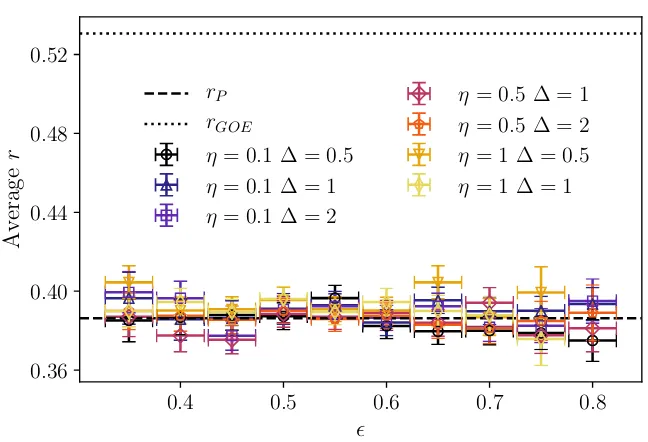
FIGURE 1.1: The phase diagram of the XXZ model (1.16)

as a function of disorder strength hand energy density ,

showing the two phases and the mobility edge. The critical disorder strength was determined from an exact

diagonali-sation study of system sizes up toL = 22. The location of

the MBL transition is determined from the spectral statis-tics (turquoise upwards-pointing triangles), entanglement entropy (red squares), fluctuations of the entanglement en-tropy (green circles), the decay of a long-wavelength spin density (blue downwards-pointing triangles), and the fluctu-ations of the half-chain magnetisation (yellow left-pointing triangles). The colour scheme indicates the scaling of the

Shannon entropy with system size (D1in the notation used

(34)

transition). The transport is subdiffusive for all disorder strengths in the

strongly interacting regime (∆ > 1), while a transition between diffusive

and subdiffusive transport exists at finiteW in weakly interacting systems

(∆ <1) [62]. This anomalous transport has been linked to long-tailed (i.e.

non-Gaussian) distributions for the off-diagonal matrix elements of local spin

operators in the ergodic phase [63]. It was found that these systems satisfy a modified version of the ETH in the subdiffusive regime, in which the scaling

of the variance of the off-diagonal matrix elements with system size requires

power-law corrections to the exponential in (1.14) [63]. Furthermore, it has

been shown that energy transport is diffusive when the disorder is weak, and the system undergoes a transition to subdiffusive transport at a finite disorder

strength (which depends on the strength of the interactions) before the MBL

transition [64–66]. Subdiffusive spin transport has also been observed in a

periodically driven Floquet version of the model, with associated long-tailed distributions of the matrix elements of local spin operators in the eigenstates

of the Floquet unitary [67]. It is interesting to note that in this system, which

does not conserve energy, the MBL phase is still present [68–72].

1.4 Signatures of many-body localisation

1.4.1 Spectral statistics

The statistical properties of a model’s eigenenergy spectrum have become

one of the key diagnostics of the MBL transition [49–52, 55, 60, 61, 66, 73–

75]. This approach to studying the properties of a system has its roots in

nuclear physics [37], and more recently has become associated with inte-grable quantum systems, where it can be used as a diagnostic of integrability

[38]. The quantities of interest are the gaps between adjacent energy levels

δn=En₋En−1, whereEnare the ordered eigenenergies of the Hamiltonian,

(35)

More recently, the gap-ratio parameter

rn= min

δn δn+1

,δn+1 δn

(1.19)

was introduced [73], which is an attractive quantity as it does not depend on the density of states (the ‘unfolding’ procedure to remove this dependence

fromδnis non-trivial [75–77]). These quantities are clearly a measure of the

level-repulsion between eigenstates. In an integrable model the extensive number of conserved quantities suppresses the level repulsion, as they split

the state space into a extensive number of independent sectors. The

eigen-states in each sector are not influenced by those in other sectors, so their

eigenenergies will not be correlated, and the distribution of level spacings can have significant weight near zero. On the other hand, in non-integrable

and non-localised models there are fewer conserved quantities to suppress

matrix elements, and the resulting level repulsion causes the distribution of level spacings to vanish at zero.

In the context of MBL we would therefore expect to find level-repulsion in

the ergodic phase and no level-repulsion in the localised phase; the transition is often located by determining the disorder strength at which this behaviour

changes. We may gain a cartoon understanding of this difference by

con-sidering a single particle on a disordered lattice. In a localised state, the

wavefunction decays exponentially in space, and therefore it has negligible

overlap with another localised state at a distance∆x ξ. The

hybridisa-tion between these states is then exponentially small, and a significant level

repulsion (i.e. repulsion on the scale of the typical level spacing) requires consecutive eigenstates to be located nearby in space, which is vanishingly

unlikely in the thermodynamic limit. We will therefore not observe the

power-law suppression of the level-gap distribution that we would see in

ergodic systems. In contrast, two extended states will necessarily have signif-icant weight on the same parts of the lattice, and the Hamiltonian may couple

(36)

MBL phase, this argument becomes that two consecutive eigenstates will

generically differ by an extensive number of eigenvalues of the LIOMs, so

the Hamiltonian cannot hybridise them to produce level repulsion on the scale of the typical level spacing [40].

To put this on a more quantitative footing, in the localised phase the eigen-energies are effectively independent random numbers, and are thus described

by a Poisson distribution:

PP(δ) = 1 αexp

−δ α

→ PP(r) = 2

(1 +r)2 (1.20)

whereαis the average level spacing. The form ofPP(r)can be derived by

showing that the ratio of two uncorrelated Poisson-distributed variables,˜r,

has the distributionPP(˜r) = (1 + ˜r)−2, and the factor of two is a result of the

contribution fromr >˜ 1, asPP(˜r−1_{) = ˜}_r2_PP_(˜_r)_.

In the thermalising phase, the level statistics have been found to follow the

statistics of a random-matrix ensemble; for models with real Hamiltonians

(such as the XXZ model in (1.16)) this is the Gaussian orthogonal ensemble

(GOE). The distribution of δ in this case is well described by ‘Wigner’s

surmise’ [78, 79]:

PGOE(δ) =βδexp(−γδ2), (1.21)

whereβandγare appropriately chosen constants. An appropriate

‘Wigner-like surmise’ has been derived forr[79]:

PGOE(r) =

27 4

r+r2

(1 +r+r2₎5/2, (1.22)

and the residual discrepancy is well captured by the correction term:

δP(r) = C (1 +r)2

r 1 +r2 −

c1r2

(1 +r2₎2

, (1.23)

(37)

c1 = 2₄π−−π4 to satisfy normalisation conditions. The averages and second

mo-ments of these distributions are shown in Table 1.1, which can be compared

to the numerical data to determine whether or not the system is localised. In Fig. 1.1 turquoise upwards triangles show the position of the MBL transition

as determined byhr_i.

Distribution hr_i _hr2_i

PP(r) ln 4−1 3−ln 16 ≈0.386294 ≈0.227411

PGOE(r) 2(2−

√

3) _≈0.351522 ≈0.535898

PGOE(r) +δP(r) ≈0.530745 ≈0.346437

TABLE1.1: Moments of the gap-ratio parameterrcalculated

from the distributions corresponding to localised and ergodic systems.

1.4.2 Entanglement

A key observation is that the entanglement across a cut in the system behaves differently in the ergodic and localised phases. The entanglement between

two parts of a system,Aand its complementB, can be quantified by the von

Neumann entanglement entropy

SvN(ρA) =−TrρAlnρA, (1.24)

whereρAis the reduced density matrix of subsystemA, found by tracing

over the degrees of freedom in subsystemBin the full-system density matrix.

The ergodic phase is characterised by long-range entanglement, so the von Neumann entanglement entropy across a cut grows with the volume of the

subsystem (i.e.∼ld_{for a subsystem of linear size}_l_{), whereas in the localised}

phase the entanglement is short-ranged, so the entanglement entropy follows

an area law (i.e. ∼ ld−1_{) [18]. It is straightforward to show that the von}

(38)

density matrix,ρ_∼exp (₋βH):

SvN(ρth) =−Trρthlnρth

=₋TrX α

1 Ze

−βEα_ln

1 Ze

−βEα

|α_ihα_|

=βX α

1 Ze

−βEα_Eα_{+ ln}_ZX

α 1 Ze

−βEα

=βE+ lnZ =βE₋βF =βT Sth

=Sth,

(1.25)

whereZis the partition function and we have setkB = 1. AsSthis extensive

in system size by definition, the area-law scaling in the localised phase clearly

signifies a failure to thermalise.

It was observed that the fluctuations in the entanglement entropy of the eigenstates have a maximum at the MBL transition, and this has become a

common diagnostic of the critical disorder strength [50, 55]. This peak can be

understood in a simple way: in the vicinity of the MBL transition, a small difference in disorder strength (or energy density, in the presence of a

mobil-ity edge) can cause the entanglement properties to change, so the variance

of entanglement entropy will diverge with system size over a window that

contains the MBL transition as it includes both extended and localised states [50]. The red squares and green circles in Fig. 1.1 show the position of the

MBL transition as determined by the scaling properties and fluctuations of

the entanglement entropy respectively.

The time-dependence of the entanglement entropy also has distinctive

fea-tures in the MBL phase. If we initialise a system in a non-entangled state

(which is not an eigenstate), and observe how the entanglement entropy across a cut depends on time, we find an unbounded logarithmic growth

with time,S_∼ln(V t), whereV is the interaction strength [80–82].

(39)

behaviour [18]. This is also distinct from the non-interacting Anderson

insula-tor, which shows no spreading of entanglement after an initial fast relaxation

[18, 81].

1.4.3 Eigenvector measures

The behaviour of the wavefunction is perhaps the most obvious indicator of

localisation, as it directly indicates the populations of individual basis states

within the eigenstates of the model. A common method in non-interacting

systems is to measure the moments of eigenstates|ψαiin the position basis

{|xi}[17]:

I_qα =X x

|hx_|ψαi|2q. (1.26)

A fully extended state will scale with the system sizeV ashx|ψαi ∼V−1/2_,

andIα

q ∼V1−q, while a localised state decays exponentially with distance, so

Iα

q ∼constant as long as the system extends beyond the localisation length.

The inverse participation ratio (IPR), defined asIα

2, quantifies the inverse

number of sites occupied by|ψαiin real space. In an ergodic state the IPR will

decay asV−1_{, but if}_Iα

2 ∼V−D2 where0< D2<1, the state is sub-extensive

in real space, and is described as delocalised but non-ergodic. We may

gen-eralise this to other moments of|ψαiasIα

q ∼VDq(1−q); if these generalised

dimensionsDqdepend onq, as is the case at the Anderson transition [3], the

eigenstate is called multifractal.

An analogous approach is taken in many-body systems, applying the idea of

localisation in state space. For an eigenstate|α_ithe moments are defined as

[17, 83]:

I_qα=X n

|hn|αi|2q∼ NDq(1−q) (1.27)

where|niis a basis with dimensionN (in a chain ofd-level systems with

lengthL, for example,_N =dL_{). For a thermalising state, we expect to see a}

result similar to that for a fully random matrix in the GOE:Iα

2 ≈3/N [83].

These quantities clearly depend on the basis chosen for|ni, and while the

(40)

is less obvious in an interacting system. To study localisation in real space

one might study the IPR of an eigenstate in the Pauli basis [83], while the

IPR of an arbitrary state with respect to the energy eigenstates is related to its survival probability [84].

Another quantity related toDqis the Renyi entropy:

S_q(R),α= 1 1₋q ln I

α q

∼DqlnN, (1.28)

and the Shannon entropy corresponds to theq_→1limit:

Sα

Sh= lim_q_→₁S(qR),α=−

X

n

|hn_|α_i|2ln_|hn_|α_i|2, (1.29)

which allows us to calculateD1 (asI1α ≡1). The colour scheme in Fig. 1.1

corresponds toD1, showing the difference in the scaling ofSShwith system

size between the ergodic and localised phases. It has been noted thatSShand

SvNexhibit very similar behaviour, but the Shannon entropy is less expensive

to calculate numerically [83].

1.4.4 Breakdown of the eigenstate thermalisation hypothesis

In a phase that fails to thermalise we can expect that operators will not be

well described by the ETH ansatz, which we can thus use to test for the MBL

phase. A key assumption of the ETH is that the expectation values of local observables taken with respect to the eigenstates of the Hamiltonian, known

as eigenstate expectation values (EEVs), are smooth functions of their

eigen-energies. Therefore examining the statistical distribution of the difference

between the EEVs of consecutive eigenstates,δhOni=hOi(En+1)− hOi(En),

offers a simple method for determining whether or not a system is localised

[48, 49, 85]. In the thermalising phase this should be peaked at zero with

a width that decreases with increasing system size [48, 86], whereas this

will not be the case in the localised phase. Considering the operatorsz

nas

an example, deep in the localised phase one would expect the eigenstates

(41)

specific disorder realisation. In this limit, the expectation values ofsz

nwill be

those of a spin either aligned or anti-aligned with the field (i.e.±1/2), with

no correlation between the values in neighbouring eigenstates. As a result,

the distribution ofδ_hsz

niwill be sharply peaked around the values 0 and±1,

which correspond to neighbouring eigenstates with the same or different

expectation values respectively.

The off-diagonal elements can also be used as a diagnostic of interesting

behaviour. While the diagonal elements of an operator describe the

aver-age values of quantities, the off-diagonal elements are associated with the relaxation to these averages. As such, the behaviour of off-diagonal elements

in the ergodic phase preceding the MBL transition has received recent

in-terest. It has been found in numerical studies that the onset of anomalous

subdiffusive transport is accompanied by a change in the distributions of off-diagonal matrix elements, which develop long tails, violating Berry’s

conjecture that the fluctuations should be Gaussian [63, 67]. This behaviour is

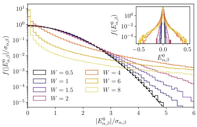
demonstrated in Fig. 1.2 [63], where the distributions are consistently Gaus-sian for all system sizes with weak disorder, but develop long tails when

the disorder is stronger. The matrix elements of spin operators in the

one-dimensional disordered XXZ model were also shown to satisfy a modified

version of the ETH, which includes a power-law correction to the exponential decay of the off-diagonal elements with system size,

hα|A|βi ∝e−s(E)L/2Lγ/2Rα,β, |Eα−Eβ|< L−γ−1, (1.30)

where the additional power-law comes from the behaviour off(E, ω)in (1.14)

[37, 63]. This power-law is related to the subdiffusive transport through the

(42)

−0.2 0.0 0.2

10−7

10−5

10−3

10−1

101 p ( h α | S

z i|

β

i

)

W =0.4 L=12

L=14

L=16

L=18

L=20

−8 −4 0 4 8

10−8 10−6 10−4 10−2 100 p ( h α | S

z i|

β

i

/σ

)

W =0.4

−0.5 0.0 0.5

hα|S_iz|βi

10−5

10−3

10−1

101 p ( h α | S

z i|

β

i

)

W =2.0 L=12

L=14

L=16

L=18

L=20

L=22

−20 ₋10 0 10 20

hα|Sz_i|βi/σ

10−8

10−6

10−4

10−2

100 p ( h α | S

z i|

β

i

/σ

)

W =2.0

FIGURE1.2: The distributions of off-diagonal elements of

sz

nin the eigenbasis of the disordered XXZ model for weak

disorder (upper panels) and stronger disorder (lower panels). The panels on the right have been rescaled horizontally by the standard deviation of the data, and the successful collapse of all system sizes onto the same curve shows that the results are indicative of the true behaviour in the thermodynamic

(43)

Chapter 2

Systems with time-dependent

parameters

When a system is affected by time-dependent parameters (i.e. when it exists

in a time-dependent environment) it adds another layer of complexity to its equations of motion. In this chapter we will discuss the effects of this

time-dependence on quantum systems, namely non-adiabatic effects caused

by a time-dependent Hamiltonian. These effects have become increasingly

prominent with the development of sophisticated cold-atom experiments in which the timescales of the dynamics can be on the order of milliseconds; this

is slow enough that it is experimentally viable to change the Hamiltonian

much faster than the system can react, and to properly probe non-equilibrium quantum effects. We will then move on to consider systems which are affected

by classical noise, both ‘white’ noise and noise with more structure in its

temporal correlations, and we will discuss the practicalities of determining

the time-evolution of such systems.

2.1 Time-evolution in quantum systems

The dynamics of a quantum system are governed by the Schrödinger

equa-tion, which describes the time-dependence of a quantum state|ψ(t)_idue to a

HamiltonianH(t):

(44)

If we define the unitary operator which evolves a state from an initial timet0

to a final timet,_|ψ(t)_i=U(t, t0)|ψ(t0)i, it follows that the unitary obeys the

same equation:

i∂tU(t) =H(t)U(t), (2.2)

whereU(t) :=U(t,0).

A generic expression forU(t)(known as a Dyson series) can be derived by

integrating (2.2) and repeatedly inserting the resulting equation into itself:

U(t) = 1₋i

Z t

0

dt0_H(t0)U(t0)

= 1₋i

Z t

0

dt0_H(t0)

"

1₋i

Z t0

0

dt00_H(t00)U(t00)

#

= 1₋i

Z t

0

dt0_H(t0)₋

Z t

0

dt0

Z t0

0

dt00_H(t0)_H(t00)

+i

Z t

0

dt0

Z t0

0

dt00

Z t00

0

dt000H(t0)H(t00)H(t000) +...

=T

∞ X

n=0

(−i)n n!

Z t

0

dt0H(t0)

n

=T exp

−i

Z t

0

dt0H(t0)

(2.3)

whereT is the time-ordering operator which dictates that the following

op-erators must act in order of increasing time, as enforced by the limits of the

integrals in the third line. The factor of1/n!in the penultimate line appears as

a result of extending the upper limits of each integration tot, which includes

then!possible orderings of thenoperators in the integrand.

2.1.1 Systems with time-independent Hamiltonians

The form ofU in (2.3) immediately suggests that for systems in which_H(t) =

H, the logical choice of basis is the eigenbasis of the Hamiltonian {|n_i}.

(45)

the unitary and quantum state at all times can be written simply as:

U(t) =X n

e−iEnt_n_n

ψ(t)=X

n

nψ(0)e−iEnt_n

(2.4)

whereEnis the energy eigenvalue of the eigenstate|ni.

2.1.2 Systems with time-dependent Hamiltonians

The problem is more complicated if we consider a system in which the

Hamil-tonianH(t)changes in time, as the eigenbasis of the Hamiltonian becomes

time-dependent and transitions between these instantaneous eigenstates are

possible. IfH(t)changes smoothly from H(0) = H(i)_to_H_(T_{) =} _H(f)_{, we}

can gain some insight by writing the state in the instantaneous eigenbasis of

H(t),_{|n(t)_i}:

ψ(t)=X

n

cn(t)n(t). (2.5)

The Schrödinger equation then gives the equations of motion for the

ampli-tudescn(t):

i∂tcn(t) =En(t)cn(t)−i

X

m

n(t)∂t

m(t)cm(t), (2.6)

whereEn(t) is the instantaneous eigenenergy of _|n(t)_i. Importantly this

has off-diagonal terms of the formhn(t)|∂t|m(t)i, which generate transitions

between the instantaneous eigenstates ofH(t). A more intuitive form of (2.6)

in terms of the time-derivative of the Hamiltonian is:

i∂tcn(t) =En(t)−in(t)∂tn(t)cn(t)

−iX m6=n

n(t)∂tH(t)

m(t)

(46)

This can be shown by taking the inner product of the time-derivative of

H(t)_|m(t)_iand_|n(t)_iwithm₆=n:

n(t)∂th_H(t)m(t)i=n(t)∂thEm(t)m(t)i

n(t)h∂tH(t)m(t)+H(t)∂tm(t)i=Em(t)n(t)∂tm(t)

n(t)h∂t_H(t)m(t)+En(t)∂tm(t)i=Em(t)n(t)∂tm(t)

n(t)∂tH(t)m(t)= (Em(t)−En(t))n(t)∂tm(t)

(2.8)

where the∂tEm(t)hn(t)|m(t)i term that would appear on the second line

vanishes due to orthogonality.

There are two simple limits where the evolution can generically be described

exactly.

The sudden limit (T _→0)

If a system is prepared in a state |ψ(0)i, and att = 0 the Hamiltonian is

instantaneously changed fromH(i)_to_H(f)_{, the system has no time to react.}

As a result, the evolution of the system can be trivially evaluated in{|nfi},

the eigenbasis ofH(f)_:

ψ(0)=X

n

niψ(0) ni=X n

nfψ(0) nf

ψ(t)=X

n

nfψ(0)e−iE(f)n t_nf_,

(2.9)

whereEn(f) is the eigenenergy of the state|nfi. Despite the apparent

sim-plicity of this limit, the study of sudden changes to the parameters of a

many-body Hamiltonian (known as a ‘quantum quench’) is an active area of

theoretical research with a rich phenomenology [87].

The adiabatic limit (T _{→ ∞})

The opposite limit, in which the Hamiltonian changes infinitely slowly with

(47)

a time-derivative, so must decrease in magnitude as T−1_{. Thus, as} _T _→

∞ the transitions between the instantaneous eigenstates of H(t) vanish,

and the system will adiabatically follow this basis. In other words, the

populations of the instantaneous eigenstates ofH(t)are constant in time, and

they accumulate a relative phase:

ψ(t)=X

n

n(0)ψ(0)e−iRt

0dt0En(t0)+iφn(t)n(t). (2.10)

The first contribution to the phase, known as dynamical phase, is a

sim-ple generalisation of the linear phase accumulation in (2.4). The second

contribution is known as geometric phase, which has the form:

φn(t) =i

Z t

0

dτ_hn(τ)_|∂τ|n(τ)i (2.11)

and results from the changing eigenbasis of the Hamiltonian. Note thatφn(t)

is a real number, so this is purely a contribution to the phase and has no effect

on the populations of levels.

2.1.3 The adiabatic theorem

The adiabatic theorem states that a quantum system in an instantaneous eigenstate will remain in that eigenstate if a perturbation acts on it

suffi-ciently slowly and if there is a gap separating the eigenenergy from the rest

of the spectrum [88]. This corresponds to theT → ∞limit discussed above,

and we shall now consider this more quantitatively to understand when the

state|ψ(t)_ican be accurately approximated by (2.10). A derivation of these

results can be found in [89].

To the next order beyond the adiabatic approximation, the probability for a

non-adiabatic transition to occur between the statesmandnis given by:

Pm→n=

Z T

0

dteiRt

0dt0(En(t0)−Em(t0))hn(t)|∂tH(t)|m(t)i

En(t)−Em(t)

2

. (2.12)

(48)

that∆En,m(t) =En(t)−Em(t)andDn,m(t) =hn(t)|∂tH(t)|m(t)iare constant

in time:

Pm→n≈

_∆EDn,m2

n,m 2

2 [1₋cos(∆En,mT)]

∼ Dn,m ∆E2 n,m 2 , (2.13)

where we have discarded the details in the second line, noting only that

2(1₋cosx)is a number of order 1 for a typical (i.e. non-fine-tuned) time

T. Assuming that∆En,m(t)andDn,m(t)are smooth functions of time, the

transition probability between these two states will generally be smaller than

Pm→n.Max

Dn,m(t) ∆En,m(t)2

2 , (2.14)

where the maximum is taken overt. The condition thatPm→n1gives us a

criterion for the validity of the adiabatic approximation. It is worth noting

that the criterion of the right-hand side of (2.14) being much smaller than one

is overly restrictive in practice, but has been used to good effect in protocols designed to minimise non-adiabatic transitions [90].

2.1.4 The Landau-Zener problem

Non-adiabatic effects are well illustrated in the Landau-Zener problem, a

time-dependent quantum system solved simultaneously by L. D. Landau

[91], C. Zener [92], E. Majorana [93], and E. C. G. Stueckelberg [94] in 1932. They considered a two-level system in which two states with an energy

difference that depends linearly on time with a ‘speed’vare coupled by a

constant parameter∆:

HLZ(t) =

vt 2σ

z₊∆ 2σ

x_, _(2.15)

whereσµ_{are Pauli matrices in the}_{|↑i_,_|↓i}_{basis. The system is initialised}

Non equilibrium processes and ergodicity breaking in isolated quantum systems

Scott Richard Taylor

A Thesis Submitted for the Degree of PhD

at the

University of St Andrews

2019

Full metadata for this item is available in

St Andrews Research Repository

at:

http://research-repository.st-andrews.ac.uk/

Please use this identifier to cite or link to this item:

http://hdl.handle.net/10023/17867

Non-equilibrium processes and ergodicity-breaking in

isolated quantum systems

Scott Richard Taylor

This thesis is submitted in partial fulfilment for the degree of

Doctor of Philosophy (PhD)

at the University of St Andrews

ergodicity-breaking in isolated

quantum systems

Acknowledgements

Contents

List of Figures

Introduction

Chapter 1

Many-body localisation

1.1

Disorder-induced localisation

1.2

Thermalisation in quantum systems

1.3

Many-body localisation in spin chains

1.4

Signatures of many-body localisation

Chapter 2

Systems with time-dependent

parameters

2.1

Time-evolution in quantum systems