An Information System for Risk Vulnerability Assessment to Flood

An Information System for Risk-Vulnerability

Assessment to Flood

Subhankar Karmakar1_{, Slobodan P. Simonovic}2_{, Angela Peck}2_{, Jordan Black}2

1_{Centre for Environmental Science and Engineering, Indian Institute of Technology Bombay, Mumbai, India} 2_{Department of Civil and Environmental Engineering, The University of Western Ontario, London, Canada}

E-mail: skarmakar@iitb.ac.in, simonovic@uwo.ca

ReceivedMay 18, 2010; revised June 20, 2010; accepted June 25, 2010

Abstract

An exhaustive knowledge of flood risk in different spatial locations is essential for developing an effective flood mitigation strategy for a watershed. In the present study, a risk-vulnerability analysis to flood is per-formed. Four components of vulnerability to flood: 1) physical, 2) economic, 3) infrastructure and 4) social; are evaluated individually using a Geographic Information System (GIS) environment. The proposed meth-odology estimates the impact on infrastructure vulnerability due to inundation of critical facilities, emer- gency service stations and bridges. The components of vulnerability are combined to determine an overall vulnerability to flood. The exposures of land use/land cover and soil type (permeability) to flood are also considered to include their effects on severity of flood. The values of probability of occurrence of flood, vulnerability to flood, and exposures of land use and soil type to flood are used to finally compute flood risk at different locations in a watershed. The proposed methodology is implemented for six major damage cen-ters in the Upper Thames River wacen-tershed, located in the South-Western Ontario, Canada to assess the flood risk. An information system is developed for systematic presentation of the flood risk, probability of occur-rence of flood, vulnerability to flood, and exposures of land use and soil type to flood by postal code regions or Forward Sortation Areas (FSAs). The flood information system is designed to provide support for differ-ent users, i.e., general public, decision-makers and water management professionals. An interactive analysis tool is developed within the information system to assist in evaluation of the flood risk in response to a change in land use pattern.

Keywords:Flood Management, Flood Risk, Geographic Information System, Risk Management, Vulnerability Analysis, Information System

1. Introduction

Records of loss of life and damage caused by floods worldwide show that these have continued to rise stead-ily during recent years. Understandably, the response has been to call for increased efforts to protect life and prop-erty. The sustainable and effective management of floods demands a holistic approach—linking socio-economic de- velopment with the protection of natural ecosystems and appropriate management links between land and water uses. It is recognized that a watershed is a dynamic sys-tem in which there are many interactions between human population, land use and water bodies. Assessment and mapping of “flood risk” [1-7] and “vulnerability to flo- od”, and dissemination of the appropriate information to different stakeholders is a very important part of the flo-

and its tributaries are assessed using a mathematical model developed for Thames Water Rivers Division, UK. The River Thames Strategic Flood Defence Initiative examines the vulnerability of floodplain development along the river. The achievements of the Flood Risk Mapping Program, New Brunswick, Canada, are sum-marized by Burrell and Keefe [9]. The procedures used to produce flood risk maps are outlined very clearly along with an assessment of the accuracy achieved. Floyd [1] performs a flood risk assessment on the city of Bombay (Mumbai), India. The results provide an initial indication of the cost-effectiveness of different remedial measures. Morris and Flavin [10] present maps of Eng-land and Wales showing the built-up areas that would be at flood risk. Shrubsole [11] mentions government re-sponsibilities in flood management of the Saguenay and Red River valley and provides alternative flood man-agement strategies considering ecosystem manman-agement, partnerships and the role of science. Hall et al. [12] represents the processes of fluvial and coastal flooding over linear flood defence systems in sufficient detail to test alternative policy options for investment in flood management. Potential economic and social impacts of flooding are assessed using national databases of flood-plain properties and demography. A case study of the river Parrett catchment and adjoining sea defences in Bridgwater Bay in England demonstrates the application of the method and presentation of results using Geo-graphic Information System (GIS). Barredo et al. [13] aims to illustrate a framework for flood risk mapping at pan-European scale produced by the Weather-Driven Natural Hazards (WDNH). The threatening natural event is represented as the hazard component, and furthermore, exposure and vulnerability are considered as anthropo-genic factors that contribute also to flood risk. The flood risk is considered on the light of exposure, vulnerability and hazard, and mathematically considered as product of hazard, exposure and vulnerability.

Vulnerability assessments have been undertaken to un- derstand the “potential for loss”, traditionally they focu- sed on the nature of the hazard and who and what are exposed [14]. More recently, vulnerability assessments have explored the social, economic, and political condi-tions that are likely to affect the capacity of individuals or communities to cope with or adapt to hazards [15]. Bender [16] discusses the development and use of natu-ral hazard vulnerability assessment techniques in the Americas. He emphasizes how and why a thorough vul-nerability analysis is required for physical, economic and social planning in a watershed. There are numerous studies that have addressed contemporary vulnerability of different communities worldwide to flooding from the natural hazards perspective of understanding exposure and the number of people and structures affected [17,18] but few that explore the socio-economic aspects of flo-

oding vulnerability [19-22]. Recently, the conceptualiza-tion on social vulnerability has gained prominence in the literature. It is related to characteristics that influence an individual’s or group’s ability or inability to anticipate, cope with, resist, and recover from or adapt to any ex-ternal stress such as the impact of flooding [23-25]. Cut-ter et al. [26] present a method for assessing vulnerabil-ity in spatial terms using both biophysical and social in-dicators. Their results suggest that the most biophysically vulnerable places do not always spatially interact with the most vulnerable populations. Flax et al. [27] develop a risk-vulnerability assessment methodology named as Community Vulnerability Assessment Tool (CVAT), which assists emergency managers in their efforts to re-duce vulnerabilities through hazard mitigation, compre-hensive land use and development planning. Cutter et al. [28] list factors that have gained consensus among social scientists as contributing to social vulnerability to envi-ronmental hazards. Blong [29] introduces a new damage index for estimating the replacement cost of damaged buildings in vulnerability analysis. Carter [30] analyzes flood risk as a combination of threat, consequence, and vulnerability. He discusses the federal role in investment decisions for flood control infrastructure. Chakraborty et al. [31] develop two new quantitative indicators, i.e., a geophysical risk index, based on National Hurricane Center and National Flood Insurance Program data, and a social vulnerability index, based on census information. Rygel et al. [32] focus on constructing a social vulner-ability index and its application to a case study of hurri-cane storm hazard. They demonstrate a method of ag-gregating vulnerability indices for different indicators using Pareto ranking that results in a composite index of vulnerability, which avoids the problems associated with assigning weights. Werritty et al. [33] discuss the social impacts of flood events in Scotland including attitude and behavior toward flooding events, warnings, evacua-tions and consequences. The study suggests ways for enhancing social resilience for sustainable flood man-agement in Scotland.

The flood risk mapping and analysis on various flood prone watersheds have been performed by many resea- rchers throughout the world. In a recent study on Roman- ian national strategy, Varga et al. [41] provide basic in-formation for preliminary flood risk assessments and flood hazard mapping in all areas with a significant flood risk, according to the Flood Directive. The technical and scientific approach and the main steps in setting up the plan for flood prevention, protection and mitigation at the river basin level are presented. Apel et al. [7] per-form flood risk analyses in Eilenburg, Germany, espe-cially in urban areas and tested a number of combina-tions of models of different complexity both on the haz-ard (probability of occurrence) and on the vulnerability. Chang et al. [42] examine the anthropogenic and natural causes of flood risks in six representative cities in the Gangwon Province of Korea. Tran et al. [43] explore the impacts of floods on the economy, environment and so-ciety; and tries to clarify the rural community’s coping mechanism to flood disasters in Central Viet Nam. They reveal that flooding is an essential element for a coastal population, whose livelihood depends on productive functions of cyclical floods. Forster et al. [44] assess flood risk for a rural detention area, alongside the Elbe River in Germany. They find that the losses in agricul-tural areas exhibit a strong seasonal pattern, and the flooding probability also has a seasonal variation. The flood risk is assessed for a planned detention area based on loss and probability estimation approaches of differ-ent time frames, namely a monthly and an annual ap-proach.

The present research study is motivated by the Hots- pots project [45,46] completed by the Center for Hazards and Risk Research (CHRR) at Columbia University and the World Bank’s Disaster Management Facility [DMF), now the Hazard Management Unit (HMU). In the Hot-spots project, the risk levels are estimated by combining hazard or probability of occurrence with historical vuln- erability for two indicators of risk—population and Gross Domestic Product (GDP) per unit area—for six major natural hazards: earthquakes, volcanoes, landslides, floods, droughts, and cyclones. The relative risks for each grid cell, rather than country as a whole, is calcu-lated at sub-national scales. Such information can inform a range of disaster prevention and preparedness measures, and development of long-term land-use plans and multi- hazard risk management strategies. Hotspots global analysis and case studies stimulate additional research, particularly at national and local levels. The present study develops an information system for risk-vulner- ability analyses to flood and facilitates vulnerability mitigation by providing various flood information to different users. The information system is designed to provide selective access to information on the bases of user needs. This reduces the misuse of data and promotes

data security. A set of suitable vulnerability indicators and the procedure for their integration into an overall vulnerability index with high spatial density represent the major analysis tool within the information system. The additional innovations of the information system include: 1) the computation of selected flood risk-vulnerability indicators organized into themes from four components of vulnerability to flood, i.e., physical, economic, infra-structure, and social vulnerability [15], 2) the spatial in-frastructure vulnerability analysis to flood due to inunda-tion of main communicainunda-tion routes and road bridges, 3) the spatial flood impacts due to inundation of critical facilities (schools, hospitals, and fire stations) and 4) quantification of exposures of land use/land cover and soil permeability to flood. The postal codes or Forward Sortation Areas (FSA) are considered for spatial discre-tization of the region and flood risk evaluation. An in-teractive analysis tool is also developed for calculation of flood risk as a function of change in land use. The pro-posed information system is implemented to six major damage centers in the Upper Thames River watershed, located in the South-Western Ontario, Canada. The study focuses only on floods which are caused by the overflow of river banks that are characteristics for the region of interest.

As a prerequisite, some relevant technical definitions are provided in the next section. The third section cont- ains a detailed description of the study area—the Upper Thames River basin in South-Western Ontario, Canada. The fourth, fifth and sixth sections provide the details on determination of probability of occurrence, vulnerability and exposures of land use and soil permeability to flood, respectively; and summarize the results obtained. The seventh section describes the features of developed in-formation system for risk-vulnerability analyses to flood. The eighth section summarizes the conclusions from the study.

2. General Definitions

the concept of Kron [50] and Barredo et al. [13], where flood risk is expressed as a function of the hazard, vul-nerability and exposed values:

) (

) ( )

( Land Soil

e V E and E

p Risk

Flood    (1)

Hazard may be defined as a threatening event, or the “probability of occurrence (pe)” of a potentially damag-ing phenomenon within a given time period and area [31, 47]. It frequently encompasses hydrological and hydrau-lic analyses and the mapping of flood lines on floodplain. Vulnerability to flood (V) is defined as a measure of a regions’ or population susceptibility to flood damages [51-53]. Exposures of land use (ELand_{) and soil}

perme-ability (ESoil_{) to flood quantify their effect on the severity}

of flood. When the exposures of land use/land cover and soil permeability to flood are considered, these denote how land use and soil permeability affects the severity of flood. For example, urbanized land use pattern results in an impervious soil layer increasing the severity of flood

and thus the exposure of land use pattern to flood in an urban area is high. The exposure of soil permeability to flood is also directly related to flood flow. The more permeable soil has more infiltration capacity and there-fore reduces surface runoff, whereas less permeable soil has less infiltration capacity and is more prone to water logging [54].

In the present study, all the information on the above mentioned three components of flood risk are effectively presented and processed using GIS. The layout for col-lecting and integrating the data, along with the sequential procedural steps for data processing and representation are outlined in Figure 1. The vulnerability section in

Figure 1, illustrates the concept of layering data using a GIS, as well as combining vulnerability components to assess the overall vulnerability to flood. The next section presents the detailed characteristics and geography of the study area.

Impact of Exposures Vulnerability

Flood Risk Assessment

Risk Components

Land Use Pattern

Soil Drainage Characteristics (Permeability) Flood Lines

- 100 yr - 250 yr

Hazard

Risk Indices

Information System

Users

Decision-Makers

Professionals General Public Physical

Vulnerability

(Descriptors – structural)

Infrastructure Vulnerability

(Descriptors - age, differential, access, household structure, social status, ethnicity, economic)

Layer 1 Layer 2

Layer P

Layer 1 Layer 2

Layer E

Layer 1 Layer 2

Layer I

Layer 1 Layer 2

Layer S

(Descriptors – biological sensitivity)

(Descriptors - critical facilities, transportation) Economic

Vulnerability

Social Vulnerability

Vulnerability to Flood

3. Study Area

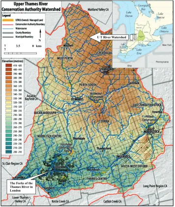
The Upper Thames river basin lies in the middle of south western Ontario; drains an area of 3,500 km2_{; and is}

populated by approximately 422,000 people. The basin is nested between the Great Lakes Huron and Erie. The basin has a well documented history of flooding events dating back to the 1700s. A detailed map of the Upper Thames River watershed in Ontario, Canada with a loca-tion map (inset) is shown in Figure 2. Two main tribu-taries of the Thames River, referred to as the North (1,750 km2_{) and South (1,360 km}2_{) branches, join at a}

location in London known as “The Forks” (Figure 2). The Forks region has served as a historical landmark for London, and is characterized by both commercial and

residential structures. Major flood damage centers in the watershed include communities of London, St. Marys, Ingersoll, Mitchell, Stratford and Woodstock. The Upper Thames river basin is an area of special importance for the sustainable socio-economic development of Ontario. This is a large and fertile area, and plays an important role in agriculture production from, fishing and aquacul-ture to perennial fruit trees. The flooding in the Upper Thames river watershed has the great effect on the fertil-ity of soil and increase in the natural aquatic production. It is also the most dangerous natural disaster hazard af-fecting the socio-economic development and the life of the people in the area. Several studies have already been done to estimate the economic damage in the watershed due to flooding [55].

U T River Watershed

The Forks of the Thames River in London

7 3.5 0 kms 7

N

The study area consists of a number of major postal code regions, some of which extend beyond the water-shed bo- undaries. The Forward Sortation Areas (FSAs) are distinguished by the first three characters of their postal code designation. The regions which historically experience more frequent flooding events are selected as areas of particular significance and the FSAs of these regions are selected for analysis. A total of 25 FSAs from these cities have been considered in the study, and are listed in Table 1. These FSAs are the smallest spatial geographic units considered in this study. The cities of important FSAs include London (17 FSAs), Woodstock (3 FSAs), Mitchell (1 FSA), St. Marys (1 FSA), Ingersoll (1 FSA) and Stratford (2 FSAs); with a particular em-phasis on the city of London. Table 1 shows that the largest FSA by area in London is N6P; with an area of 103 km2 and in the entire study area is N0K; with an area of 1510.0 km2_{. The smallest FSA by area in London is}

N6B; with an area of 3.2 km2_{, and in the entire study}

area is N4Z; with an area of 0.5 km2_{. The average area of}

an FSA in London is 29.5 km2 and the average area of all FSAs in the study area is 122.2 km2_.

Numerical data necessary for the development of a flood information system has been collected from Statist- ics Canada, which provides updated national statistics consistently every five years following a Census of the population. Data is available for areas of various sizes, including FSAs as small census divisions which remain relatively stable over many years. Various layers and datasets compatible with the GIS software are collected from Statistics Canada, The Ontario Fundamental Data-set, Upper Thames River Conservation Authority (UTR- CA), Surficial Geology of Southern Ontario (SGSO) dataset, and Route Logistics (RL). These datasets are available online or obtained from the Serge A. Sawyer map library and the Internet Data Library System (IDLS) at the University of Western Ontario (UWO), London, Canada. Table 2 presents the detailed information on different data layers with their formats and sources used in the present case study. All three components of the flood risk are assessed and represented in the information system separately in dissimilar ways. Each component is represented graphically, numerically, or using a combi-nation of both. Next two sections describe the method-ologies for determination of probability of occurrence and vulnerability to flood.

4. Probability of Occurrence

Probability of occurrence of flood (pe) [31] describes a physical threat from a flood occurring and a region beco- ming inundated. The consideration of probability of occu- rrence as a flood risk component is essential, since flood

Table 1. List of the municipalities and FSAs (PSEPC* 2005).

Municipality FSA _{(in km}Area 2₎ Municipality FSA _{(in km}Area 2₎

N5V 46.7 N6L 38.0

N5W 15.7 N6M 28.7

N5X 27.0 N6N 70.0

N5Y 10.0

London

N6P 103.0

N5Z 11.0 Mitchell N0K 1510.0

N6A 7.1 N4S 326.0

N6B 3.2 N4T 4.1

N6C 13.5

Wood- Stock

N4V 2.1

N6E 20.6 St. Marys N4X 327.0

N6G 25.8 N4Z 0.5

N6H 41.5 Stratford N5A 233.0

N6J 12.0

London

N6K 28.4 Ingersoll N5C 149.0

*Public Safety and Emergency Preparedness Canada.

Table 2. Information on data layers used in GIS.

Indicator Source* Layer Type

Wetlands OFD wetlands_unit Polygon

Roads OFD road Line

Railways OFD transport_line Line

Unpaved roads OFD road Line

Intersections RL ren Point

Critical facilities OFD building_symbol Point

Bridges RL rll Line

Land use RL ONland_use Polygon

Soil permeability SGSO sgu_poly Polygon

100-year flood line UTRCA -- Line

250-year flood line UTRCA -- Line

Grid BM obmindex Polygon

FSAs RL zip Polygon

*OFD—Ontario Fundamental Dataset (OGDE-Alymer_Guelph.mdb) from the Serge A. Sauer Map Library at UWO; RL—CanMaps Route Logistics, 2006 dataset from the UWO IDLS; SGSO—Surficial Geolo- gy of Southern Ontario, 2003 cd-rom dataset from Serge A. Sauer Map Library aUWO; UTRCA—the layers obtained from the Upper Thames River Conservation Authority in 2007; BM—Ontario Base Map Sheet, 2001 from the UWO IDLS.

risk of a highly vulnerable population to flood is neglig- ent if there is less probability or chance of occurrence of flood. The probability of occurrence (i.e., the extreme events and associated probability) of flood is also termed as “flood hazard” by many researchers [7,13,47,50,56]. In the present study however, the available results on pe

The probability or likelihood of occurrence of flooding is described as the chance that a location will be flooded in any one year. For example, 1.3% chance of flooding each year implies 1 in 75 chance of flooding at that loca-tion in any year. Exceedance probability (pe) of a flood is represented as [31,57]:

) ( 1 ]

[X x p F x

P   e   (2)

where F(x) denotes the value of Cumulative Distribution Function (CDF) of river flow x. The return period (Tx) of flood flow x is the reciprocal of exceedance probability, which is mathematically represented as [57]:

)] ( 1 /[ 1 ] [ /

1 P X x F x

Tx     (3)

A flood line of a particular return period is the extreme boundary of the region exposed to a flood of the same re- turn period. It represents the spatial extent of threat from the flood of a particular return period. The flood lines for a particular return period are evaluated by using physical, hydraulic and hydrologic characteristics of a particular location in the watershed. The present study utilizes 250- year flood line data for all FSAs being considered and 100-year flood line data for FSAs within the City of Lon- don, as per the availability. A flood hazard map with 100 and 250-years flood lines is used as one of risk compon- ents depicting spatial extent of flooding with exceedance probability of 0.01 and 0.004, respectively. The follow-ing procedural steps are followed in GIS for incorporat-ing the information on probability of occurrence in this study: 1) the FSA, 100 and 250-years flood line shapefile layers are imported into ArcMap [58]; 2) the FSA layer and 100-yr flood line layers are turned “on” so that they are displayed in the Data Viewing window; 3) twenty five FSAs of interest in this study are highlighted using the selection tool and then converted into their own layer (FSA layer of interest); 4) these map features are then observed in the “layout” view where it is possible to in-sert map elements such as north arrows, legends and scale bars using the Insert Map Elements feature; 5) the map is then exported to “.jpeg” format. The same proce-dure is repeated for the 250-year flood line layer.

5. Vulnerability to Flood

Vulnerability to flood is defined as measure of a region’s susceptibility to flood damage [51-53]. It also includes population susceptibility to physical, mental or emotional damage due to flooding. Vulnerability could be influen- ced by individual emotions, seriousness of the current situation, and previous experiences with natural disasters. Traditionally, vulnerability has considered only biophy- sical factors. More recently, social factors have also been incorporated into assessment of vulnerability to disasters [31].

In this study, vulnerability to flood has been defined as

a combination of four distinctive types of vulnerabilities: physical, economic, infrastructure and social [15]. The

physical vulnerability generally incorporates only those indicators susceptible to biological sensitivity. Wetlands are for example, considered regions of physical vulnera- bility in this study. Wetlands are among the most produ- ctive ecosystems on earth. The richness of these transi-tional ecosystems relates mostly to the diversity of eco-logical niches created by the variability of seasonal and interannual cycles. Modifications in the hydrologic re-gime that disturb these cycles have been found to be the main stress factor threatening shoreline wetlands in all the world's major rivers [59]. The regulation of water levels has also caused the shrinkage of wetlands, and an incidental reduction in the diversity of plant communities and the number of plant species [60]. These regions have high biodiversity and sensitive life, which would experi-ence higher damages, longer, slower recovery times due to flooding. Economic vulnerability includes flood dam-age indicators which can be expressed in monetary terms.

Infrastructure vulnerability includes civil structure such as road networks, railways, and road bridges. Infrastruc-ture components are important to movement of popula-tion, communications, and safety. Their inundation im-pedes traffic and hinders communications, increasing stress in the exposed population. Inundation may also block important emergency routes and cause physical damage to roads. Social vulnerability focuses on the re-action, response, and resistance of a population to a dis-astrous event. Vulnerable population may require special attention in an evacuation situation for example. The indicators are chosen based on a review of existing lit-erature assessing vulnerability to current hazards [25-27, 31,32,51].

The vulnerability index (VIi) corresponding to each indicator for ith _{FSA is calculated using the following}

equation, which standardizes [61] each vulnerability in-dex value ranging from 0.0 to 1.0 as done by Wu et al. [51]:

min max

min

V V

V V

VIi i _



 (4)

where Vmin _{and V}max _{are the minimum and maximum}

values of the indicator for all FSAs, respectively, and Vi

is the actual value of the indicator for ith _{FSA. All}

cial vulnerability maps are created in ArcMap on the basis of calculated values of vulnerability indices. The following procedure is followed for calculating the sum of the length of roadways/railways: 1) roads/railways layer is imported into GIS; 2) the length of each road/railway is contained in the attributes table; 3) those road/railway segments from the attribute table are se-lected which fall within and intersect a particular FSA; 4) the “statistics” option from the “length” field in the at-tribute table options is selected; 5) the program calcu-lates the sum of lengths and display them in that particu-lar FSA; 6) the values are stored in a table and finally 4) is used for determining the vulnerability indi-ces—“length of roads” and “length of railways”. The similar procedure is followed for the vulnerability in-dex—“unpaved roads”, but the unpaved, dirt and gravel roads are selected for each FSA individually using the “Select by Location” or “Select by Attributes” tool.

This calculation of vulnerability index using 4) [61] offers an improvement over the traditional calculation [26,31,51] of vulnerability index, i.e., dividing all values by the maximum value, _VI (_{V V}max)

i

i  , as it considers

both the maximum and minimum values and ensures that the vulnerability indices are within [0, 1] interval and always non-negative. It is not necessary to use the scale [0, 1] for standardization. Montz and Evans [25], Grosshans et al. [54] and Odeh et al. [62] standardize the values of vulnerability and plotted the maps considering [0, 10], [0, 5] and [0, 100] scales, respectively. In the assessment of infrastructure vulnerability, the present study considers: a) the impact of flooding of critical fa-cilities (schools, hospitals, and fire stations) and b) the spatial impact of flooding of main communication routes and road bridges. The developed methodologies for con-sidering these impacts are discussed in next two subsec-tions. The main objectives of the analysis presented in these two subsections are: 1) to model the impact of in-undation of critical facilities (e.g., schools, hospitals and fire stations) of an FSA on its total infrastructure vulner- ability, which is achieved by considering the “number of critical facilities (i.e., number of schools or hospitals within an FSA)” as vulnerability indicators [determined by using 4), as done for physical, economic, social and other infrastructure vulnerability indicators]; and 2) to model the impact of inundation of an FSA (which may contain one or more than one critical facilities) on its surrounding FSAs, which is modeled using a grid system. There are numerous studies that have addressed the im-pact of inundation of critical facilities on infrastructure vulnerability based on the number of critical facilities within an FSA [27,51,62], but none that explore the im-pact on surrounding FSAs, because people dwelling out-side the flooded FSA also may depend on the critical facilities situated within the flooded FSA. This impact on infrastructure vulnerability of surrounding FSAs is

mod-eled using a grid system.

5.1. Infrastructure Vulnerability Due to Inundation of Critical Facilities

Vulnerability of critical facilities is an indicator of infra-structure vulnerability [27,51,62]. Emergency shelters, nursing homes, public buildings, schools, hospitals, fire and rescue stations, police stations, water treatment or sewage processing plants, utilities, railroad stations, air-ports and government facilities are identified as critical facilities by Odeh et al. [62] and Flax et al. [27]. Critical facilities are those that play an integral role in public safety, health, and provision of aid [27]. As per the availability of data, the critical facilities considered in this study include schools, fire stations and hospitals, and are given special attention in vulnerability analysis in order to provide a more accurate estimate of flood risk.

Schools can be used for both education and as a place of refuge and a center for aid distribution during a flood. Fire stations provide the source of response to an emer-gency in the area near the station, and aid in disaster re-lief. Flooding of a fire station causes the population in close proximity to be more vulnerable. Hospitals repre-sent another type of critical facilities that require special attention during flooding. Hospitals may have patients that need special attention in the case of an emergency. Procedure for assessment of infrastructure vulnerability due to inundation of critical facilities includes the use of a GIS tool. As per the availability of data, the FSAs of London are considered for the demonstration of the methodology. The impact of inundation of critical facili-ties of an FSA on its total infrastructure vulnerability is determined by considering the “number of critical facili-ties (i.e., number of schools or hospitals within an FSA)” as vulnerability indicators [determined by using 4), as done for physical, economic, social and other infrastruc-ture vulnerability indicators]. To model the impact of inundation of an FSA (which may contain one or more than one critical facilities) on its surrounding FSAs, a 6x6 grid layer is placed over the FSAs of London, which breaks the entire city into 36 cells, as illustrated in Fig-ure 3(a). The size of each grid cell is 25 km2 _{(5 km × 5}

The presence of just one of these is sufficient to classify the cell as important. All “important” cells are equally important. The DI values indicating vulnerability levels decrease equally in all directions with the distance from the inundated cell. Procedure implemented using GIS tool is as follows:

1) Divide the area under consideration into a grid—the grid should be regular in shape. In this analysis, a 6  6 square grid is used for demonstration purpose.

2) Use the DI to quantify the importance of a critical facility for each FSA. Red, orange, yellow and white color codes correspond to 1.0, 0.75, 0.2 and 0.0 DI val- ues, respectively. The colors are reflecting the DI of each cell: red (high), orange (medium), yellow (low), white (no influence), which indicates the importance of the pre- sence of critical facilities. The grid cells within an FSA that contain one or more critical facilities are identified. These grid cells are assigned red color, the highest DI of 1, assuming that the people closest to the facility are

its primary users.

3) Assign a white color, indicating “zero” DI value to the remaining grid cells. The result is a square-shaped representation of vulnerability, which decreases with distance from the red (center) cell.

4) Following the previous three steps, assign DI values for all grid cells separately for each case of a grid cell with red color. For example, if 10 (ten) grid cells contain critical facilities, the grids cells would be assigned ap-propriate DI values 10 times. Finally, the Overall DI (ODI) for a grid cell is calculated by averaging these ten DI values.

5) The vulnerability for an FSA—area shown in bold solid line in Figure 3(c) —is calculated as:

th

1 1

i FSA ( )

i

k k

e k k k

j j

Vul of ODI A A

 







where ODIk is overall DI for kth _{grid cell, Ak is the area of}

ith _FSA.

A1 A2

A3 _A

4

A5 A6

G1 G2

G3 G4

G5 G6

(a)

LEGEND ---- Grid line

Ak Area under kth _{grid cell} Gk kth _{grid cell with over all degree of}

importance, ODIk

N6P N6K

N6H N6G

N5X

N5Y N5V

N6M N5W N5Z N6C N6J

N6L N6N N6E 6A

6B

(b)

(c)

(d)

(e)

6) Determine the standardized vulnerability index val- ue using:

min max

min

e e

e e std

e _{Vul Vul}

Vul Vul

Vul i

i _



 (6)

where Vulemax _{and Vule}min_{are the maximum and minim-}

um vulnerability values of critical facilities, Vule_i is the

value of vulnerability for critical facilities pertaining to the ith _{FSA. Thus the standardized infrastructure}

vulner-ability values are obtained at FSA level.

5.2. Infrastructure Vulnerability Due to Inundation of Road Bridges

The infrastructure vulnerability is also affected by the inundation of road bridges. Vulnerability of an area due to the inundation of a bridge includes the interruption of traffic and formation of communication barriers between different locations in the affected region. Inundation of, or damage to a particular bridge affects not only the FSA in which it is located, but also all other FSAs that depend on the use of the bridge. In this study, only bridges over the water bodies are considered significant, because the- se bridges have limited alternate routes associated with them, and are necessary for safe crossing of the water body. They are frequently used as means for transporting commercial goods, a route to and from the workplace, and as emergency routes in case of a disaster.

The impact of inundation of road bridges of an FSA on its total infrastructure vulnerability is modeled by con- sidering the “number of road bridges” as vulnerability indicator [determined by using 4), as done for physical, economic, social and other infrastructure vulnerability indicators]. To model the impact of inundation of an FSA (which may contain one or more than one road bridges) on its surrounding FSAs, the same procedure (steps 1 through 6) as described in previous subsection is followed, with the use of the new vulnerability shapes as shown in Figures 3(d) and (e). Again, 6  6 grid is used in the assessment of vulnerability as shown in Figure 3(a). However, the shape used in assessing vulnerability due to the inundation of road bridges is not a box, but rather cross-like. The shape varies with the number of bridges in any particular grid cell. Figures 3(d) and (e)

illustrate the shapes of vulnerability for cells containing 1-5 and 6-10 road bridges, respectively. The number of bridges over water that is contained in each cell deter-mines the shape that would be used in assessment of vulnerability. As the number of bridges increases, the more likely it is that inundation of that cell would affect more people. The vulnerability shape due to inundation of bridges is mainly based on a basic assumption: the need for crossing any given bridge decreases with dis-tance from the bridge (i.e., the need for crossing the

bridge is highest in areas that are closest to the bridge), because people further away from a particular bridge may have other alternatives for crossing the water body with equal convenience. The proposed method assumes that the whole cell being considered is flooded, and that bridges in that cell are unavailable for use. The cells are assigned a DI based on the vulnerability mapping in proximity to the inundated cell. The DI assignment is similar to the one used in assessing the infrastructure vulnerability due to inundation of critical facilities. However, the road bridges scenario designates a DI as either red/high (1.0) or yellow/low (0.2) for demonstra-tion of the proposed methodology. In both analyses it was assumed that the whole grid cell is equally affected by the flooding, thus damage is assumed to be uniform across the cell area. The population density within a por-tion of the FSA covered by a grid cell is not known. Therefore a uniform distribution of population is as-sumed throughout each FSA.

The following procedural steps are followed in GIS for incorporating the information on infrastructure vuln- erability due to inundation of critical facilities: 1) the “buildings” layer is imported; 2) in the attribute table the type of building is specified. In the options for the attrib-ute table “select by attribattrib-ute” is used and then the cate-gory (e.g., school/hospital/fire station) is used to select only those buildings which are schools/hospitals/fire stations; 3) these buildings are saved as a separate layer for referencing in the critical facilities analysis of the study. The same procedure is followed for road bridges but the “bridge” layer is imported.

The calculation of the vulnerability indices following the procedures described in this section provides input for mapping each category of vulnerability in GIS. Table 3 shows the values of four components of vulnerability in the Upper Thames River basin. The seventh column of

“so-cial status” and “ethnicity”.

The present study incorporates a unique consideration of inundation of road bridges and critical facilities in ass- essing infrastructure vulnerability.

Figure 4 displays the difference in infrastructure vul-nerability due to inundation of critical facilities and road bridges. In most cases, the standardized values of infra-structure vulnerability of the FSA increase with the addi-tion of impacts due to the inundaaddi-tion of road bridges and critical facilities. The GIS generated map may be produ- ced for each component of vulnerability values as pre-sented in Table 3 for identifying spatial variability of vulnerabilities to flood. More details of the processed numerical data and graphical results of the present vul-nerability analysis to flood can be obtained from Peck

et al. [63].

5.3. Calculation of the Vulnerability to Flood

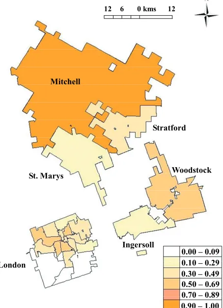
Although maps of individual component of vulnerability can be useful, it is easiest to assess vulnerability throug- hout the watershed if the multidimensional components can be integrated into a single measure [32]. In the pres- ent study, the simplest way to combine the four compo- nents of vulnerability into a single measure would be to average the values of indices [31,51] for each component [as given in the seventh column of Table 3]. Figure 5

shows the GIS generated map of vulnerability to flood obtained by averaging and standardizing the four comp- onents of vulnerability. The darker color indicates larger vulnerability. Map in Figure 5 provides for easy comp- arison of vulnerability between different FSA regions of six major damage centers, and insight into the spatial

Table 3. Vulnerability analysis to flood of the Upper Tham- es River basin.

Components of Vulnerability to Flood Damage

Center FSA

Phy. Eco. Infras. Soc.

Overall vul* Rank

N6A 0.000 0.264 0.432 0.383 0.296 15 N6B 0.000 0.282 0.467 0.399 0.316 12 N6C 0.014 0.613 0.477 0.794 0.498 6 N6E 0.000 0.128 0.256 0.767 0.303 13 N6G 0.000 0.495 0.556 0.703 0.471 9 N6H 0.015 0.828 0.356 0.784 0.503 5 N6J 0.000 0.876 0.447 0.732 0.296 14 N6K 0.004 0.457 0.299 0.613 0.527 4 N6L 0.000 0.000 0.022 0.000 0.353 11 N6M 0.009 0.234 0.172 0.012 0.000 25 N6N 0.044 0.004 0.055 0.020 0.110 19 N6P 0.005 0.084 0.089 0.072 0.032 22 N5V 0.002 0.815 0.305 0.813 0.061 20 N5W 0.000 0.515 0.421 0.608 0.486 8 N5X 0.034 0.288 0.293 0.390 0.405 10 N5Y 0.001 0.707 0.461 1.000 0.268 16 London

N5Z 0.005 0.539 0.502 0.736 0.562 3 Michell N0K 1.000 0.749 1.000 0.632 1.000 1

N4S 0.000 1.000 0.510 0.715 0.572 2 N4T 0.000 0.110 0.011 0.082 0.041 21 Wood-stock

N4V 0.004 0.027 0.008 0.030 0.010 23 St. Marys N4X 0.002 0.266 0.299 0.181 0.200 18

N4Z 0.000 0.048 0.000 0.021 0.009 24 Stratford

N5A 0.134 0.673 0.384 0.690 0.494 7 Ingersoll N5C 0.092 0.293 0.275 0.261 0.249 17

*Overall vulnerability: standardized average values

0 2 4 8 12 16

Kilometers

N6P N6K N6H

N6G N5X

N5Y N5V

N6M N5W

N5Z N6C N6J

N6L

N6N N6E

N6A

N6B

N6P N6K N6H

N6G N5X

N5Y N5V

N5W

N5Z N6C N6J

N6L

N6N N6E

N6A

N6B

N6M

0.00 – 0.09 0.10 – 0.29 0.30 – 0.49 0.50 – 0.69 0.70 – 0.89 0.90 – 1.00 (a) (b)

variability of vulnerability. It is identified from Table 3

and Figure 5 that FSA–N0K in Michell is the most vul-nerable in the basin, as the area under this postal code is much larger than other FSAs and consequently it con-tains a number of wetlands and more infrastructure. It is found that the vulnerability values for FSAs in London vary between 0 and 0.562. The FSA–N5Z is identified as the most vulnerable, whereas N6M is identified as the least vulnerable within the city of London. The Table 3

and Figure 5 give a general description of region’s vul-nerability, and can be used for emergency flood man-agement, disaster mitigation activities and planning fu-ture disaster protection infrastrucfu-ture.

It should be noted for clarification that, there may be some correlation among vulnerability indicators under different components of vulnerability. In this study the chance of involving correlated indicators is very less, as the indicators are chosen based on a review of existing literature [25-27,31,32,51]. If the number of indicators is too high Principal Components Analysis (PCA) [32] can be applied to select the set of uncorrelated indicators. The basic aim of a PCA is to reduce a complex set of many correlated variables into a set of fewer, uncorre-lated components.

London

Ingersoll Mitchell

Woodstock Stratford

St. Marys

12 6 0 kms 12

0.00 – 0.09 0.10 – 0.29 0.30 – 0.49 0.50 – 0.69 0.70 – 0.89 0.90 – 1.00

Figure 5. GIS generated map of standardized average vuln- erability to flood.

6. Exposures of Land Use and Soil

Permeability to Flood

The present study utilizes 250-year flood line data for all FSAs and 100-year flood line data for FSAs within the City of London, as obtained from UTRCA, Canada, for considering the values of probability of occurrence in the calculation of flood risk. The impacts of land use and soil type are not considered during generation of the flood lines and probability of occurrences. To incorporate the impact of exposures of land use and soil permeability into the analysis a separate component of the flood risk is considered as expressed in (1), following Kron [50] and Barredo et al. [13]. The indices of vulnerability to flood, as discussed in previous section, have no influence on flood flow and river channel characteristics. The expo-sures of land use and soil permeability are two physical watershed characteristics which affect the flood flow [64], and are considered as the important characteristics of flood risk in the Upper Thames River watershed. This study considers the impact of exposures of land use and soil permeability only for those FSAs within the munici-pality of London as per the availability of data. An ex-posure value of 1 is assigned to the regions outside of the City of London.

6.1. Land Use

The land use map used in the present study is obtained from the UWO Internet Data Library System (IDLS). Their CanMap Route Logistics 2006 dataset contains the Ontario land use GIS layer. This layer is designated as “ONland_use” and is of type “polygon” as mentioned in

Table 2. The available land use data include seven dif-ferent categories of use: open space, commercial, resi-dential, parks and recreational, government and institu-tional, resource and industrial, and water body. Each of these land use categories has been assigned a DI value. These values, while estimated by the research team, can be changed by decision-makers with more extensive kn- owledge on how different land use influences flood run-off characteristics. Overdeveloped and highly commer-cialized areas include more pavement and impervious surfaces. They increase runoff quantity and shorten the time of concentration. On the other side, open land (in-cluding agricultural land) is exposed to direct infiltration of rainfall which decreases runoff quantity and lengthens the time of concentration. With this knowledge, the DI values are assigned to each category of land use, which are as follows: water body (0.1), parks & recreational (0.2), open area (0.3), Government and institutional (0.7), commercial (0.8), residential (0.8), resources & indus-trial (0.8).

each type multiplied by its DI provides an exposure value representative of the land use for an FSA. There-fore, mathematically the exposures of land use to flood for ith _{FSA is expressed as:}

)] / ( [ 1 i l i n l l Land

i DI A A

E 





(7)

where Land i

E is the exposure of land use to flood, DIl is the DI of land use type “l”. “l” may be any of the land use types. Area under each land use type l is expressed as

Al

i for ith FSA. Total area of the ith FSA is denoted as Ai.

6.2. Soil Permeability

Soil permeability refers to the hydrological drainage cha- racteristic of soil to allow water movement through its pores, which is inversely proportional to soil density. The more permeable the soil is, the more water can be transmitted through it. A soil with low permeability, such as clay, doesn’t permit much water flow. This could ca- use “puddling” of water and thus higher accumulation of water on the soil surface. Regions which are composed primarily of these types of soils are prone to a higher flood risk because the water requires a longer time to drain or infiltrate into the ground [54]. Using a GIS dataset known as Surficial Geology of Southern Ontario, it was possible to spatially assess the soil permeability characteristics of the region. The data is available with different designations of permeability: low, medium-low, high or variable. A DI is assigned to each permeability category based on the ability of soil to infiltrate water, facilitate its transmission, and decrease flooding. DI val-ues assigned to each category of soil permeability are as follows: low (0.8), low-medium (0.6), variable (0.5), high (0.3).

Area under each permeability category is expressed as a fraction of the FSAs total area. Summation of the frac-tion of each category multiplied by its DI provides an exposure value representative of soil permeability for an FSA. Therefore, mathematically the exposure of soil permeability to flood for ith _{FSA is expressed as:}

)] / ( [ 1 i p i m p p Soil

i DI A A

E 





(8)

where Soil i

E is the exposure of soil permeability to flood,

DIP is the DI of permeability category “p”. “p” may be low, medium-low, variable and high. Area under each permeability category (p) is expressed as p

i

A for ith _FSA.

Total area of the ith _{FSA is denoted as Ai. The}

standardi-zation is being performed following the equation similar to (4) and (6), expressed as:

min max min E E E E Estd i

i _



 (9)

where Emax _{and E}min_{are the maximum and minimum}

ex-posure values pertaining to land use/soil permeability, Ei

is the value of exposure of land use/soil permeability pertaining to the ith _{FSA. The following procedural steps}

are followed in GIS for incorporating the information on exposures of soil permeability and land use to flood: 1) the Ontario Surficial Geology dataset for Zone 17 in On-tario is imported into ArcMap; 2) the layer features are symbolized by categorical attributes; 3) to symbolize each soil type with its own colour, the Layer Properties dialogue box is opened, “Symbology” and “Categories” tabs are selected from the left menu, and “unique values” is highlighted; 4) in the Value Field, “SINGLE_PRI” is selected, which represents the single primary material of the soil composition. A colour scheme is selected and then each soil is represented by its own colour in the ArcMap data viewer; 5) the “Select by Location” tool of GIS is used to isolate those soils which fall within a par-ticular FSA; 6) an area calculation is then performed on these “soils of interest” which provides the area of each soil type and the FSA boundaries that the soil area is within. An additional field is entered into the layers at-tribute table; the name of the field (column) and its type (floating point, integer etc.) are specified. All values are initialized to 0. The calculator option is then selected to compute the areas of the selected attributes. An advanced Visual Basics Application (VBA) area statement is used to calculate the required areas; 7) the type of each soil can be found in the layers attribute table along with the soils characteristic permeability which varied from “low” to “high”; 8) the results are summarized in a table. A similar procedure is followed for land use, but “cate-gory” is symbolized by: Commercial, Government & Institutional, Open area, Parks and Recreational, Resi-dential, Resource and Industrial, and Water body. The impacts of exposures of land use and soil permeability to flood for FSAs of London are tabulated in Table 4. All

Table 4. Impact of exposures of land use and soil perme-ability to flood.

Impact of Exposures (standardized value) FSA

Based on land use Based on soil permeability

N6A 0.7362 0.2139

N6B 1.0000 0.0000

N6C 0.7562 0.9403

N6E 0.4311 0.9497

N6G 0.3954 0.5836

N6H 0.2481 0.5144

N6J 0.7067 0.8668

N6K 0.3339 0.4643

N6L 0.0000 1.0000

N6M 0.0386 0.7239

N6N 0.0125 0.9149

N6P 0.0122 0.7982

N5V 0.3049 0.3906

N5W 0.7427 0.1372

N5X 0.2357 0.3267

N5Y 0.8250 0.2760

the values are standardized with in [0, 1] to produce an indicator scores. Table 4 indicates that the exposure of land use for FSA-N6B, which is located in the central part of London, has maximum impact to flood due to presence of more commercial, residential and industrial areas; whereas the exposure of soil permeability has minimum impact to flood, as N6B has high permeable soil with high drainage capacity. The table also indicates that the exposure of land use for FSA-N6L, which is lo-cated in the southern part of London, has minimum im-pact to flood due to presence of more open and recrea-tional areas; whereas the exposure of soil permeability has more impact to flood, as N6L has low permeable soil with less drainage capacity.

7. Development of the Information System

Providing a website for people to access flood risk infor- mation is an effective way of informing the public about the susceptibility to flooding that they may otherwise not be aware of. The study of Barredo et al. [13] is a contri-bution to the discussion about the need for communica-tion tools between the natural hazard scientific com- mu-nity and the political & decision making players in this field. The website can serve as an information center and may provide analysis tools for interactive processing of available flood information. It also provides the opp- ortunity to tailor the presentation of the same information to different types of users according to their needs.Acc- ording to the program evaluation glossary of USEPA [65], an information system is an organized collection, storage, and presentation system of data and other know- ledge for decision making, progress reporting, and for planning and evaluation of programs. It can be either manual or computerized, or a combination of both. The information from the present risk-vulnerability analysis to flood is systematically kept in a computerized inform- ation system for more efficient use. The Adobe Dreamw- eaver Creative Sweet 3 software (http://www.adobe.com/ ap/products/dreamweaver) is used for creating the flood information system. The whole website is based off the Cascading Style Sheets (CSS) template provided in Adobe CS3. The developed information system is easy to navigate. The process starts by providing access to dif-ferent FSAs of 6 damage centers in the Upper Thames watershed. After selecting the damage center, typing in the first three digits of an FSA will direct the user to in-formation about that FSA. Selected three digits of the FSA activate the search engine that is created using a search engine composer. Information page is available for every FSA region. The information that is displayed for all the users; includes maps, numerical data, and an analysis tool in Microsoft excel spreadsheet format for calculation of flood risk as a function of change in land use. After typing the first three digits of an FSA in an

identified cell of the spreadsheet, the user will be di-rected to the information on flood risk of the FSA, con-sidering the present land use pattern and area under dif-ferent categories of land use. Area under each land use type can be changed by the user to find out the flood risk under future scenario of land use pattern. It will calculate risk by using (1).

The prototype information system created for this risk- vulnerability analysis to flood targets 3 different user categories: 1) general public, 2) decision-makers and 3) water management professionals. The general public has access to a simple explanation of flood risk terminology, tables providing values of vulnerability to flood and a de- scription of what they mean, 100-year and 250-year flo- od lines, as well as a simple analysis tool for flood risk calculation. Decision-makers are provided with a more detailed description of flood risk terminology and the implications of flooding. They have access to the same flood hazard maps as the general public. Decision-mak- ers are provided with a more detailed and flexible analy-sis tool which allows the user to change the land use and compare the present level of flood risk with the one ob-tained under changed land use scenario. This may assist in the analyses of different land development initiatives and their consequences on flood risk. Water management professionals are presented with the most detailed de-scriptions and the most technical flood related informa-tion. They are provided a very detailed numerical break-down of vulnerability and exposures of land use and soil permeability, including a list of all indicators used in the analyses. They also have access to the flood hazard maps similar to those provided to the general public and the decision-makers. The analysis tool available to professio- nals is the same as one provided to the decision-makers. The professionals are the only user with access to a “raw data” containing all of the numerical data used for the flood risk analyses. Screenshots of the opening page of prototype information system and analysis tool are shown in Figures 6(a) and (b). The information system is user-friendly and the details can be found in Black

et al. [66].

8. Conclusions

(a)

(b)

number of critical facilities and road bridges. Typically, exposures of land use and soil permeability have been included as a component of risk. The minimum and max- imum values of vulnerability are considered in the stand- ardization process instead of using the conventional for- mula for standardization. A user-friendly information sys- tem is designed to systematically represent all flood info- rmation. The study provides an “analysis tool” for estima-tion of flood risk as a consequence of change in land use. The present study has some limitations and offers so- me benefits for future development. In the flood inform- ation system all the indices of infrastructure vulnerability for critical facilities are not considered due to unavaila- bility of data. For example, emergency shelters, nursing homes, public buildings, police stations, water treatment or sewage processing plants, utilities, railroad stations, airports and government facilities; which are identified critical facilities [27,62]. The assignment of Degree of Importance (DI) for calculation of impact inundation of important service buildings, emergency service stations and road bridges across the river on infrastructure vuln- erability, and in calculation for exposures of land use and soil permeability is dependent on the perspective of deci-sion-makers or floodplain planners, which introduces some uncertainty due to vagueness or imprecision in the model. This uncertainty due to imprecision in the assi- gnment of DI may be addressed in the flood risk calcula- tion. In the present system only two flood lines are ava- ilable, e.g., 100- and 250-years flood lines, which limit the calculation of flood risk. The impact of critical facili- ties and road bridges across the river on infrastructure vulnerability is calculated only for the City of London as per the availability of data. The same analysis may be performed for other damage centers in the watershed. In future studies, different shapes and sizes of “vulnerabil- ity shapes” with finer grid system and actual population density can be considered for determining the impact of inundation of critical facilities and road bridges. The impact of climate change is not considered in the current version of the system. The hazard maps or the position of flood lines will change if the climate change impacts are taken into consideration [67]. The values of flood risk for different postal codes may be easily updated to include the impact of climate change. No hydrologic calculation is performed in the present study to find out current posi-tion of flood lines. A sophisticated hydrologic modeling may be implemented for finding out the current positions of flood lines and result in more accurate calculation of flood risk. The proposed methodologies of flood risk ma- pping are not limited to the present case study and may be easily applied to other watersheds.

9. Acknowledgements

The authors sincerely thank the Upper Thames River Co-

nservation Authority, Statistics Canada, Canadian Hom- ebuyers Guide, Serge A. Sawyer map library & the IDLS library at The University of Western Ontario for provid-ing data used in this study. Work presented in this paper has been conducted under the research grant by the Natu- ral Sciences and Engineering Research Council of Canada.

10. References

[1] P. J. Floyd, “Reducing Flood Risks,” Floods and Flood Management, 1992, pp. 419-435.

[2] E. J. Plate, “Flood Risk and Flood Management,” Journal of Hydrology, Vol. 267, No. 1-2, 2002, pp. 2-11.

[3] A. Becker and U. Grünewald, “Disaster Management: Flood Risk in Central Europe,” Science, Vol. 300, No. 5622, 2003, p. 1099.

[4] D. P. Loucks, J. R. Stedinger, D. W. Davis and E. Z. Stakhiv, “Private and Public Responses to Flood Risks,” International Journal of Water Resources Development, Vol. 24, No. 4, 2008, pp. 541-553.

[5] M. J. Purvis, P. D. Bates and C. M. Hayes, “A Probabilis-tic Methodology to Estimate Future Coastal Flood Risk Due to Sea Level Rise,” Coastal Engineering, Vol. 55, No. 12, 2008, pp. 1062-1073.

[6] R. J. Dawson, L. Speight, J. W. Hall, S. Djordjevic, D. Savic and J. Leandro, “Attribution of Flood Risk in Ur-ban Areas,” Journal of Hydroinformatics, Vol. 10, No. 4, 2008, pp. 275-288.

[7] H. Apel, G. T. Aronica, H. Kreibich and A. H. Thieken, “Flood Risk Analyses—How Detailed do We Need to be?” Natural Hazards, Vol. 49, No. 1, 2009, pp. 79-98. [8] P. Garrett, “Assessing Flood Risk,” Water Bull, Vol. 355,

1989, p. 9.

[9] B. Burrell and J. Keefe, “Flood Risk Mapping in New Brunswick: A Decade Review,” Canadian Water Resour- ces Journal, Vol. 14, No. 1, 1989, pp. 66-77.

[10] D. G. Morris and R. W. Flavin, “Flood Risk Map for England and Wales,” Report - UK Institute of Hydrology, 1996, p. 130.

[11] D. D. Shrubsole, “Flood Management in Canada at the Crossroads,” Global Environmental Change Part B: En-vironmental Hazards, Vol. 2, No. 2, 2000, pp. 63-75. [12] J. W. Hall, R. J. Dawson, P. B. Sayers, C. Rosu, J. B.

Chatterton and R. Deakin, “A Methodology for National- scale Flood Risk Assessment,” Proceedings of the Insti-tution of Civil Engineers: Water and Maritime Engineer- ing, Vol. 156, No. 3, 2003, pp. 235-247.

[13] J. I. Barredo, A. de Roo and C. Lavalle, “Flood Risk Mapping at European Scale,” Water Science and Tech-nology, Vol. 56, No. 4, 2007, pp. 11-17.

[14] S. L. Cutter, (Ed.) “American Hazardscapes: The Re-gionalization of Hazards and Disasters,” Joseph Henry Press, Washington, D.C., 2001, p. 211.

[16] S. Bender, “Development and Use of Natural Hazard Vulnerability-Assessment Techniques in the Americas,” Natural Hazards Review, American Society of Civil En-gineers, 2002, pp. 136-138.

[17] L. Roy, R. Leconte, F. Brissette and C. Marche, “The Im- pact of Climate Change on Seasonal Floods of a Southern Quebec River Basin,” Hydrological Processes, Vol. 15, No. 3, 2001, pp. 3167-3179.

[18] N. Nirupama and S. Simonovic, “Increase in Flood Risk Due to Urbanization: A Canadian Example,” Natural Hazards, Vol. 40, No. 1, 2007, pp. 25-41.

[19] M. Morris-Oswald and S. Simonovic, “Assessment of the Social Impacts of Flooding for Use in Flood Management in the Red River Basin,” Report Submitted to the Interna-tional Red River Basin Task Force, InternaInterna-tional Joint Commission, Winnipeg, Manitoba, 1997. http://www.ijc. org/php/publications/html/assess.html

[20] E. Enarson, “Women, Work, and Family in the 1997 Red River Valley Flood: Ten Lessons Learned,” Disaster Pre- paredness Resources Centre, University of British Co-lumbia, British CoCo-lumbia, Canada, 1999.

[21] E. Enarson and J. Scanlon, “Gender Patterns in Flood Evacuation: A Case Study in Canada’s Red River Val-ley,” Applied Behavioural Science Review, Vol. 7, No. 2, 1999, pp. 103-124.

[22] Natural Hazard Center, “Evaluation of a Literature Re-view of the Social Impacts of the 1997 Red River Flood,” Report Submitted to the International Red River Basin Task Force, International Joint Commission. University of Colorado, Boulder, Colorado, USA, 1999, p. 11. [23] P. Blaikie, R. Cannon, I. Davis and B. Wisner, “At Risk:

Natural Hazards, People’s Vulnerability, and Disasters,” Routledge, New York, 1994, p. 284.

[24] P. M. Kelly and W. N. Adger, “Theory and Practice in Assessing Vulnerability to Climate Change and Facilitat-ing Adaptation,” Climatic Change, Vol. 47, No. 4, 2000, pp. 325-352.

[25] B. Montz and T. Evans, “GIS and Social Vulnerability Analysis,” In: E. Gruntfest and J. Handmer, Eds., Coping with Flash Floods, Kluwer Academic Publishers, Neth-erlands, 2001, pp. 37-48.

[26] S. L. Cutter, J .T. Mitchell and M. S. Scott, “Revealing the Vulnerability of People and Places: A Case Study of Georgetown County, South Carolina,” Annals of the As-sociation of American Geographers, Vol. 90, No. 4, 2000, pp. 713-737.

[27] L. K. Flax, R. W. Jackson and D. N. Stein, “Community Vulnerability Assessment Tool Methodology,” Natural Hazards Review, American Society of Civil Engineers, Vol. 3, No. 4, 2002, pp. 163-176.

[28] S. L. Cutter, B. J. Boruff and W. L. Shirley, “Social Vul-nerability to Environmental Hazards,” Social Science Quarterly, Vol. 84, No. 2, 2003, pp. 242-261.

[29] R. Blong, “A New Damage Index,” Natural Hazards, Vol. 30, No. 1, 2003, pp. 1-23.

[30] N. T. Carter, “Flood Risk Management: Federal Role in Infrastructure,” CRS Report for Congress, 2005, http://

fpc. state.gov/documents/organization/56095.pdf [31] J. Chakraborty, G. A. Tobin and B. E. Montz,

“Popula-tion Evacua“Popula-tion: Assessing Spatial Variability in Geo-physical Risk and Social Vulnerability to Natural Haz-ards,” Natural Hazards Review, American Society of Civil Engineers, Vol. 6, No. 1, 2005, pp. 23-33.

[32] L. Rygel, D. O’Sullivan and B. Yarnal, “A Method for Constructing a Social Vulnerability Index: An Applica-tion to Hurricane Storm Surges in a Developed Country,” Mitigation and Adaptation Strategies for Global Change, Vol. 11, No. 3, 2006, pp. 741-764.

[33] A. Werritty, D. Housto, T. Ball, A. Tavendale and A. Black, “Exploring the Social Impacts of Flood Risk and Flooding in Scotland,” Scottish Executive Social Re-search, Edinburgh, 2007.

[34] S. K. Sinnakaudan, A. Ab Ghani, M. S. S. Ahmad, and N. A. Zakaria, “Flood Risk Mapping For Pari River Incor-porating Sediment Transport,” Environmental Modelling and Software, Vol. 18, No. 2, 2003, pp. 119-130.

[35] J. Bai, C. Wang, Z. Niu, S. Qi and G. Li, “Utilizing Re-mote Sensed TM Images and Meteorological Data to Plan Flood Risk Area,” Proceedings of The International So-ciety for Optical Engineering, Vol. 5232, 2006, pp. 370- 377.

[36] F. Forte, L. Pennetta and R. O. Strobl, “Historic Records and GIS Applications for Flood Risk Analysis in the Salento Peninsula (Southern Italy),” Natural Hazards and Earth System Science, Vol. 5, No. 6, 2005, pp. 833-844. [37] R. Abdalla, C. V. Tao, H. Wu and I. A. Maqsood, “GIS-

Supported 3D Approach for Flood Risk Assessment of the Qu’Appelle River, Southern Saskatchewan,” Interna-tional Journal of Risk Assessment and Management, Vol. 6, No. 4-6, 2006, pp. 440-455.

[38] D. G. Hadjimitsis, “The Use of Satellite Remote Sensing and GIS for Assisting Flood Risk Assessment—A case study of Agriokalamin Catchment Area in Paphos-Cy-prus,” Proceedings of The International Society for Op-tical Engineering, Vol. 6742, No. 67420Z, 2007.

[39] K. Smith, “Environmental Hazards: Assessing Risk and Reducing Hazards,” 3rd Edition, Routledge (Taylor & Francis Group), New York, 2001, p. 392.

[40] J. Lowry, H. Miller and G. Hepner, “A GIS-Based Sensi-tivity Analysis of Community Vulnerability to Hazardous Contaminants on the Mexico/U.S. Border,” Photogram-metric Engineering & Remote Sensing, Vol. 61, No. 11, 2005, pp. 1347-1359.

[41] L. A. Varga, D. Radulescu and R. Drobot, “Romanian National Strategy for Flood Risk Management,” IAHS- AISH Publication, Vol. 323, 2008, pp. 75-86.

[42] H. Chang, J. Franczyk and C. Kim, “What is Responsible for Increasing Flood Risks? The Case of Gangwon Prov-ince, Korea,” Natural Hazards, Vol. 48, No. 3, 2009, pp. 339-354.