Measuring West Africa Ports Efficiency Using Data Envelopment Analysis

(1)

ISSN Print: 2160-0473

DOI: 10.4236/jtts.2019.93018 May 30, 2019 287 Journal of Transportation Technologies

Measuring West-Africa Ports Efficiency Using

Data Envelopment Analysis

Bomboma Kalgora

1*

, Sidoine Yao Goli

2

, Bomboma Damigou

3

, Hamadou Tahirou Abdoulkarim

1

,

Kwame Kwadu Amponsem

4

1_{School of Economics and Management, Shanghai Maritime University, Shanghai, China} 2_{School of Management, Wuhan University of Technology, Wuhan, China}

3_{Institut Supérieur de Management, Dakar, Senegal}

4_{Regional Maritime University, Department of Transport, Accra, Ghana}

Abstract

The present study measured the relative efficiency of five major commercial ports in West Africa, using three different Data Envelopment Analysis (DEA) methods, the CCR, BCC, and Windows I-C methods over the years 2005-2016. Seven input variables and one output variable were used in the model analysis. The CCR and BCC methods were used to evaluate the technical and scale ef-ficiency while the Windows I-C method provided a comprehensive ranking of the studied ports. The results showed that the scale efficiency score of 89.53% indicated that on average the production scale of the ports had de-viated from the most productive scale size (MPSS) by 10.47%. These results revealed that the source of the overall inefficiency is due to scale rather than pure technical inefficiency. Hence, in order to improve the overall efficiency, the two scaled inefficient ports of Abidjan and Cotonou should adjust their scale of operations. Then, further investigations were conducted to detect correlations between various variables used in this study. The research found that the absence of any correlation for non-significant variables and negative correlation for the significant variables throughout time resulted from the fact that these variables were not fully utilized. Meaning that they were not effi-ciently used to boost the container throughput on a scale basis, the research also found that a pandemic or insecurity could easily impact seaports activi-ties with the case of the Ebola outbreak which strucked the West African re-gion from the year 2013 to 2016, or the terrorism threats which prevailed in the region around the year 2012. Thus, for ports to stand out in the present fiercely competitive environment, ports authorities ought to analyze their op-erational scale to identify whether or not the production size is fitting before further port capacity expansion.

How to cite this paper: Kalgora, B., Goli, S.Y., Damigou, B., Abdoulkarim, H.T. and Amponsem, K.K. (2019) Measuring West-Africa Ports Efficiency Using Data Envelopment Analysis. Journal of Trans-portation Technologies, 9, 287-308.

https://doi.org/10.4236/jtts.2019.93018

Received: April 6, 2019 Accepted: May 27, 2019 Published: May 30, 2019

http://creativecommons.org/licenses/by/4.0/

(2)

DOI: 10.4236/jtts.2019.93018 288 Journal of Transportation Technologies

Keywords

Container, Ports, Analysis, Scale Efficiency, Technical Efficiency, Data Envelopment Analysis, West Africa

1. Introduction

1.1. The Maritime Transport and Ports

(3)

2016) [8]. Henceforth, maritime transport is favored by the relocation of pro-duction units away from consumer markets. It comprises three basic elements such as the infrastructure of ports and container terminals, the ships and feeders that connect the seaports and lastly the systems that ensure the efficient opera-tion of equipment and infrastructure. The maritime ports, in general, constitute one of the links in the multimodal transport chain. This research aims at the commercial maritime ports of five West Africa countries, Benin, Ivory Coast, Ghana, Nigeria, and Togo. The commercial seaports are the point of intersection of bi-directional goods flow in terms of import and export.

1.2. Background of West Africa Ports

West African ports of Ivory Coast, Ghana, Togo, Benin, and Nigeria are viewed as the most competitive and developed ports and they serve as the major gate-ways for the landlocked countries (LLCs) of West Africa (Kalgora B., 2019) [9]. In relatively close distance to each other, they have witnessed significant devel-opment in the past two decades. According to a study conducted by Van de Voorde, E. & Winkelmans, W. (2002) [10] a port range is a geographically de-fined area comprising ports that serve much the same customers. West Africa is bordered by the Sahara Desert in the north with the Ranishanu Bend considered the northernmost part of the region. To the south and west, the Atlantic Ocean borders the region. The area covers approximately 5 million square kilometres (MOW, 2015) [11] with a population of approximately 340 million and a GDP per capita of USD 2500 (ECOWAS, 2015) [12]. According to the AFDB (2015) [13], the West African region had a development rate of 6% in 2014. It is at the centre of the African continent economic and financial transformation. It is the quickest developing region in Africa and this growth is depicted in a wide range of divisions crosswise over various member states. In the most recent decades, maritime trade especially container trade has experienced an impressive growth rate along with increased demand for transport logistics services. The West African container throughput has expanded on average by 10% on yearly basis (Kalgora B., 2019) [14] with the populace and the GDP average growth at 3% and 11% respectively (van Dyck G. K., 2015) [15].

(4)

2. Review of Literature on Port Efficiency and Productivity

Prior to containerization, the general cargo was handled by geared breakbulk vessels docked at piers that extended into the water. After the Second World War, with a significant increase in international trade, most ports around the world faced the problem of congestion. Cargoes were carried as breakbulk until the first load of containerized goods in 1966. They were shipped to Rotterdam and official-ly marked the beginning of containerization of international trade (Talley W. K., 2009) [2]. With advances in shipbuilding, associated cargo unitization systems were developed to reduce loading/unloading times at ports (Monteiro M., 2014) [16]. Consequently, this major breakthrough in the industry, led to the building of non-geared vessels, by redesigning containerships that would take advantage of economies of scale. Therefore in the same line of advancement in the indus-try, ports aspiring to handle more containers have had to invest more resources in quayside cranes, infrastructure and other related mobile capital.

According to Notteboom T. & Rodrigue J. (2008) [17], there are three major phases in the container freight distribution system across the history of contai-nerization internationalization. They are consequently as follows: The first phase, which is the introduction of containerization and its combination with maritime transport systems. As a result, this also led to efficiency improvements in port transshipment and inland service that became reliant on trucking. The second phase, which was more fundamental, related to the combination of con-tainerization with inland transport systems including road and rail transport. Intermodal transport systems began to emerge in the late 1970s, thus leading to the development of a new generation of ports strongly influenced by containeri-zation and intermodal transport. At that point in time, ports of which a huge part of functioning was based on information technology start emerging as lo-gistics centres. The third phase is the current stage at which ports operate. They acting as functional nodes in supply chains through containerization propelled by intermodality. Ports have become super-efficient and more competitive with regards to costs and services.

2.1. Port Efficiency

(5)

DOI: 10.4236/jtts.2019.93018 291 Journal of Transportation Technologies [22]. Efficiency is defined by the Steering Committee for the Review of Com-monwealth/State Service Provision as, the success with which organizations use an optimal amount of resources to produce outputs at a specific level of quality (Padilla M. & Eguia R., 2010) [23]. Efficiency can be broken down further in terms of its technical and allocative nature.

2.1.1. Technical Efficiency

The Technical Efficiency (TE) represents the ability of a firm to minimize the waste by producing much output as technology input usage needed or utilizing as little input needed by technology and output production (Fried et al., 2008) [24]. Similarly, Padilla & Eguia R. (2010) [23], explain that TE is the conversion of physical inputs (such as the services of employees and machines) into outputs relative to best practice. Thus, a firm or an organization operating at best prac-tice is said to be 100 percent technically efficient. If operating below best pracprac-tice levels, then the firm’s technical efficiency is expressed as a percentage of best practice (Anguibi C. F. C., 2015) [25]. Technical efficiency can be either in-put-oriented or outin-put-oriented; the choice of measurement depends on the particular nature of the industry. In the container port sector, port authority and the terminal operator can influence the production level through the use of commercial policies and different market strategies, but the provision of infra-structure is difficult to change over a short-term period. This led to the use of an output-oriented measure that features the maximum output able to be reached for a given input-mix (Liu Q., 2010) [20].

2.1.2. Allocative Efficiency

Coelli T. (1996) [26] explains that Allocative Efficiency (AE) is the ability of a firm to use the inputs in optimal proportion. Therefore, a firm can be said to be allocatively efficient when the inputs, given their prices, are used in a proportion that minimizes the cost of production. AE, similar to TE, can also be expressed as a percentage. A firm using its inputs in optimally obtaining a score of 100 percent. Cullinane K.W.F., et al., (2006) [27] state that in a competitive envi-ronment, ports should efficiently utilize their existing facilities in serving their customers, i.e., ports should ensure that the utilization of their current infra-structure, equipment and resources are economically and technically optimized. This will result in enhanced service quality by ultimately reducing vessel waiting time and translating into cost savings in the supply chain.

2.2. Port Productivity

(6)

termi-DOI: 10.4236/jtts.2019.93018 292 Journal of Transportation Technologies

nals, in particular, terminal operations involve the number of cranes available for use (how much loading/unloading is operationally possible) and crane per-formance (number of movements per crane per hour). For shipping lines, termi-nal operations are crucial to their overall operations since it affects the time ships spend at the port. Another component of performance includes the movement of cargo within the container yard. In container yard, operations are based on the terminal capacity, containers are stacked and container density is checked at a particular rate. For an efficient container yard performance, the appropriate space and equipment are essential as well as a proper organization because inef-ficient yard operations can affect the time duration trucks will spend at the yard.

2.3. Efficiency and Productivity Measurement in Port Sector

Several methodologies have been used with the aim of analyzing port efficiency and providing useful information for port development planning and strategy. The most widely used productivity and efficiency measurement approaches in-clude the Data Envelopment Analysis (DEA). The application of the DEA me-thod to the port industry is not new. Different variations of the DEA technique have been used to analyze port production in various regions worldwide. The advantages of the DEA method is that multiple inputs and outputs can be added to the model, and therefore has the capability of providing an overall evaluation of port performance (Wang T.F., et al., 2003) [28].

2.3.1. DEA for Multi-Objective Analysis

A range of studies have used the DEA model to assess efficiencies of ports at a specific point in time, either utilizing the DEA CCR or BCC models (van Dyck G.K., 2015) [22] in West Africa; (Anguibi C. F. C., 2015) [25] in West and Cen-tral Africa. Such studies have proved useful in identifying relationships between efficiency in ports and management policy-related issues, and the structures of the port. Authors like Martinez-Budria E., et al., (1999) [29] examined the effi-ciency of 26 ports in Spain using DEA-BCC models. They found that high com-plexity ports are associated with high efficiency. Utilizing both DEA-CCR and DEA-Additive models, (Tongzon J., 2001) [30] analyzed the efficiency of 4 Aus-tralian ports in addition to 12 other international container ports for the year 1996.

2.3.2. DEA Efficiency over Time

(7)

DEA window analysis model was then used to evaluate changes in container terminal efficiency over a period of 4 years for 11 terminals (Min H., & Park B., 2005) [33]. The input data used included total quay length, the number of cranes, labor force, and container yard size, in addition to container throughput as the output. Al-Eraqi A.S., et al., (2008) [34] performed two DEA analyses, a simple DEA and a DEA window analysis concerning 22 ports located in the Middle-East and East-African region from 2000 to 2005. Their researches have used both panel-data and cross-sectional data and compared efficiency in terms of the scale of ports. They concluded that larger ports are often inefficient due to decreasing return to scale while smaller ports are more efficient for the opposite reason.

Efficiency has been addressed by port-related literature from many different perspectives (Ancor S-A., et al., 2016) [35]. Essentially, port efficiency analyses established relationships between inputs mainly a port’s physical facilities and its labor force and outputs such as port throughput. In summary, the DEA model has been used extensively in port and terminal efficiency studies. There is a sig-nificant trend toward the use of the model to identify areas of inefficiency in both cross-sectional and panel data. Most studies have identified the usefulness of similar outputs and inputs for ports or terminals concerned. This ensures the model results are consistent and valid.

3. Data and Methodology

3.1. Data Collection Techniques and Data Sources

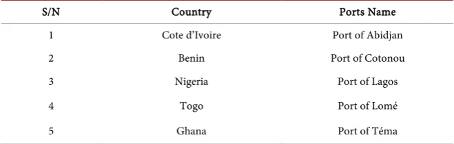
The study covers a period of 12 years from 2005 to 2016. The present research paper selected the 5 strategic countries container ports in the West African re-gion. These container ports are identified as Decision Making Units (DMUs) and are shown in Table 1 for this purpose. They practically possess similar op-erational measures.

[image:7.595.209.539.606.711.2]

The competitive analysis of these ports is carried out using the DEA Window I-C method. This method can be a useful tool for port managers and for re-searchers, providing a deeper insight into ports performances (Roll Y. & Hayuth Y., 2006) [36]. Researches revealed an absence of consensus in the choice of the type of variables (inputs and outputs) used in the DEA model (Tongzon, J., 2001) [30]. Plainly, Cullinane K. P., & Wang T.-F. (2006) [37] emphasize that the

Table 1. DEA decision making units.

S/N Country Ports Name

1 Cote d’Ivoire Port of Abidjan

2 Benin Port of Cotonou

3 Nigeria Port of Lagos

4 Togo Port of Lomé

5 Ghana Port of Téma

(8)

precise choice of inputs and output variables is critical to the evaluation of con-tainer ports terminals and undefined variables may lead to misleading conclu-sions about ports evaluation.

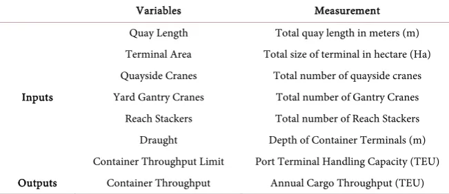
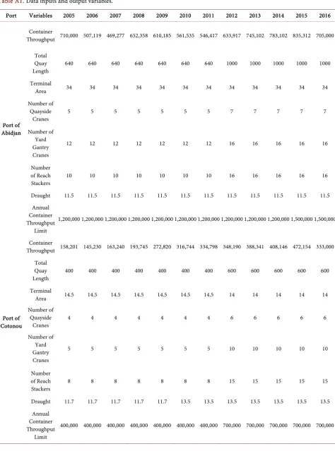
[image:8.595.210.536.570.711.2]

The research, therefore, intends to assess the operational efficiencies of the se-lected DMUs. Seven input variables and one output variable are sese-lected, and the standard container size or TEU is used with regards to the output variable (see Table 2). In order to be consistent with the production framework, like in the previous studies applying DEA method (Munisamy, S. & Singh, G., 2011) [38] (Anguibi C. F. C., 2015) [25], this research uses proxies to evaluate the port's competitiveness through the labour and capital inputs. As for the labour inputs, the number of handling equipment’s such as quayside cranes, yard gantry cranes and reach stackers, are used as proxies. The quay length, the container through-put limit, the terminal area, and the draught are selected as proxies for capital, whereas, the container throughput is used as the only output in the study.

The inputs variables data listed in Table 2 (for data, see Appendix Table A1) were compiled from national and regional ports authorities association such as the Port Management Association of West & Central Africa (PMAWCA., 2017) [39] while the output variable of each of the five DMUs, the container through-put (for data, see Appendix Table A1), is obtained from international institu-tions such as the World Bank (2017) [5], and for accuracy purpose, are double checked with other regional institutions namely the ECOWAS, and the WAEMU.

3.2. DEA Mathematical Formulation and Objective Function

The linear programming technique is used to find the set of coefficients (u's and

v's) that will give the highest possible efficiency ratio of outputs to inputs for the service unit being evaluated (Sherman H.D., & Zhu J., 2006) [40].

DMUj= service unit number j

j = number of decision making units (DMU) being compared in the DEA analysis.

θ =efficiency rating of the decision making unit being evaluated by DEA.

Table 2. DEA inputs and output variables.

Variables Measurement

Inputs

Quay Length Total quay length in meters (m) Terminal Area Total size of terminal in hectare (Ha) Quayside Cranes Total number of quayside cranes Yard Gantry Cranes Total number of Gantry Cranes

(9)

DOI: 10.4236/jtts.2019.93018 295 Journal of Transportation Technologies yij = amount of output r used by service unit j.

xij= amount of input r used by service unit j.

i = number of inputs used by the DMUs.

r = number of outputs generated by the DMUs.

ur= coefficient or weight assigned by DEA to output r.

vi = coefficient or weight assigned by DEA to input i.

The function is subject to the constraint that when the same set of u and v co-efficients is applied to all other service units being compared, no service unit (DMUs) will be more than efficient than 1. Charnes A., et al. (1978) [41] sug-gested the following mathematical programming for estimating the relative effi-ciency score of a particular DMU j among similar n entities being evaluated.

1 1 2 2 1

1 1 2 2 ₁

1, 1, , s

r rj

j j r rj r

j m

j j i ij _i _{i ij} u y

u y u y u y

DMU j n

v x v x v x v x

= = + + + = = ≤ = + + +

∑

 

 (1)

, , 0 and , , 0; 1, , ; 1, ,

r s i m

u _ u > v _ v ≥ r= _ s i= _ m

To solve the fractional mathematical programming problem, Equation (1) has been transformed into a linear programming model as written below:

1 1 1 0 1 s.t. max

0, 1, ,

1 , 0 S r ro r m r rj i ij

r i m i i i r i S u y

u y v x j n

v x u v = = = = − ≤ = = ≥

∑

 ₍₂₎

To obtain the solution of Equation (3), the dual form has been considered and presented as follows:

1

0, 1,

min

,

0, 1, ,

0, 1,

t

, s. . n ij j io

j n

rj j ro j

j

x x i m

y y r s j n θ λ θ λ λ = = − ≤ = − ≥ = ≥ =

∑

   (3)

The CCR model given above follows an input-oriented approach that is the minimization of resources for a desired amount of outputs. The present study adopted an output-oriented approach in order to determine how a port could ef-ficiently increase its throughput from a particular quantity of resources. Similar to the input-oriented CCR model formulation, the output-oriented CCR dual form is shown as follows in the Equation (4):

0 1

1

0, 1, ,

max s

0, 1, ,

0 ,

.

, ,

t

1 . n ij j i

j n

rj j ro

j

x x i m

(10)

Here φ is the value of the relative efficiency score for each DMU being eva-luated. By assuming that not all the decision-making units are operating at an optimal scale, the constraint presented below is added to the CCR, which is also called constant return to scale (CRS) model. This was conceived in order to ob-tain the BCC known as variable returns to scale (VRS) model introduced byBanker R.D., et al., (1984) [42].

1 1

n j j

λ =

=

∑

(5)

The inverse of the estimated score of φ gives the efficiency value for each DMU in both CCR and BCC model. By analyzing the efficiency of the DMUs under VRS assumptions, the scale efficiency (SE) of each DMU has been esti-mated using the efficiency scores obtained under CCR and BCC models. In fact, the efficiency observed under the CRS model is the overall measure of technical and scale efficiency; while the one deriving from the VRS model is pure technical efficiency (PTE). Hence, scale efficiency is calculated as follows in Equation (6):

TE SE

PTE

= ₍₆₎

When SE equals to 1 this indicates scale efficiency and less than one demon-strates scale inefficiency. After the estimation of scale efficiency, the nature of returns to scale has been investigated to determine whether the scale inefficiency is related to either increasing (IRS) or decreasing (DRS) returns to scale. In order to find the nature of returns to scale, a comparison is made between the effi-ciency value given by a BCC model and the one calculated under the non-increasing returns to scale (NIRS) model. According to researchers, if the efficiency value of NIRS model is different from the BCC efficiency score, thus the DMU being assessed will exhibit increasing returns to scale. In the case both efficiency indices are equal, then the particular DMU experiences decreasing re-turns to scale (Banker R.D., et al., 2004) [43]. The NIRS model is obtained by adding the restriction written in Equation (7) instead of the constraint displayed in Equation (5) in the CCR model in Equation (4).

1 1

n j j

λ =

≤

∑

(7)

As mentioned above, the standard DEA models CCR and BCC give the same efficiency value of 1 to all the efficient DMU. Consequently, it is not possible to identify among the efficient DMUs, the best performer. In order to provide ranking among the efficient ports, the window I-C is used with a windows length of 1.

4. Empirical Results

(11)

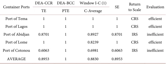
pure technical efficiency scale efficiency and the nature of returns to scale and the C-average for the five container ports under study. The results are summa-rized in Table 3.

The efficiency estimates of the CCR model is that the ports of Lagos, Lomé, and Tema are equal to 1, revealing that these ports define the best practice fron-tier in terms of technical efficiency and performance. The efficiency scores of the remaining ports are less than 1, demonstrating that they are relatively inefficient compared to the best practices ports. Considering the efficiency scores are de-rived from the BCC model, it is found that in addition to the efficient ports identified under the CCR model, the port of Abidjan and Cotonou have their ef-ficiency score equal to 1. This indicates that they are efficient in terms of re-source utilization. Therefore, among the five studied ports, three, the ports of Tema, Lagos, and Lomé are efficient in the constant returns to scale (CRS), whereas the two remainings ports, Abidjan and Cotonou are operating efficient-ly under variable returns to scale (VRS). The average efficiency value obtained from the CRS model is 89.53%, which is less than the average efficiency score es-timated in the VRS model. The average scale efficiency scores, 89.53% which in-dicates that on average the ports actual scale of production has deviated from the most productive scale size (MPSS) by 10.47%. On the whole, the results reveal that the source of the overall inefficiency is due to scale rather than pure tech-nical inefficiency.

[image:11.595.210.541.585.716.2]

The ports of Lagos, Lomé, and Tema are scale and technically efficient with a score of 1. Hence, these ports were operating at an optimal scale. Conversely, the ports of Abidjan and Cotonou, of which the efficiency scores are less than 1 in the CCR model, are efficient under BCC model. This demonstrates that they are technically efficient but scale inefficient. In other words, the ports were efficient in the utilization of input resources but they are either too small or too large re-garding the activities they perform. Hence the two scaled inefficient ports Abid-jan and Cotonou should adjust their scale of operations in order to move to-wards efficiency. Nevertheless, looking at the C-average compilation, from the Window I-C model, window 1, it is seen that out of the five ports, only two ex-hibit value equal to 1, Tema and Lagos.

Table 3. Efficiency results derived from DEA methods.

Container Ports DEA-CCR DEA-BCC Window I-C (1) SE _{to Scale Evaluation}Return

TE PTE C-Average

Port of Tema 1 1 1 1 CRS efficient

Port of Lagos 1 1 1 1 CRS efficient

Port of Abidjan 0.8701 1 0.8927 0.8701 IRS inefficient

Port of Lome 1 1 0.8239 1 CRS efficient

Port of Cotonou 0.6063 1 0.6981 0.6063 IRS inefficient

AVERAGE 0.8953 1 0.8830 0.8953

(12)

The results derived from the analysis of the nature of returns to scale are summarized in the right-most column of Table 3. The outcome highlight is that three ports exhibited constant returns to scale (CRS). In addition, the two other ports are operating at increasing returns to scale, due to their small size of pro-duction and they need to enhance their efficiency by selecting a scaling up strat-egy, which would increase their scale of operations.

5. Ports Variables Analysis

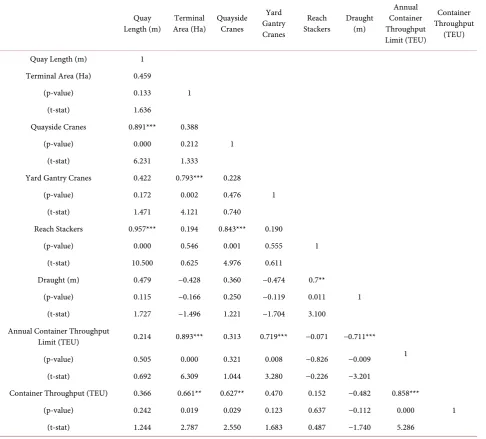
[image:12.595.59.546.274.713.2]

A close look at the correlation matrix in Table 4 reveals a highly positive corre-lation between several variables: the quayside cranes and the quay length, be-tween the quay length and the reach stackers, bebe-tween terminal area and the

Table 4. DEA correlation coefficients in year 2016.

Quay

Length (m) Area (Ha) Terminal Quayside Cranes

Yard Gantry Cranes

Reach

Stackers Draught (m)

Annual Container Throughput Limit (TEU)

Container Throughput

(TEU)

Quay Length (m) 1

Terminal Area (Ha) 0.459

1

(p-value) 0.133

(t-stat) 1.636

Quayside Cranes 0.891*** 0.388

1

(p-value) 0.000 0.212

(t-stat) 6.231 1.333

Yard Gantry Cranes 0.422 0.793*** 0.228

1

(p-value) 0.172 0.002 0.476

(t-stat) 1.471 4.121 0.740

Reach Stackers 0.957*** 0.194 0.843*** 0.190

1

(p-value) 0.000 0.546 0.001 0.555

(t-stat) 10.500 0.625 4.976 0.611

Draught (m) 0.479 −0.428 0.360 −0.474 0.7**

1

(p-value) 0.115 −0.166 0.250 −0.119 0.011

(t-stat) 1.727 −1.496 1.221 −1.704 3.100

Annual Container Throughput

Limit (TEU) 0.214 0.893*** 0.313 0.719*** −0.071 −0.711***

1

(p-value) 0.505 0.000 0.321 0.008 −0.826 −0.009

(t-stat) 0.692 6.309 1.044 3.280 −0.226 −3.201

Container Throughput (TEU) 0.366 0.661** 0.627** 0.470 0.152 −0.482 0.858***

1

(p-value) 0.242 0.019 0.029 0.123 0.637 −0.112 0.000

(t-stat) 1.244 2.787 2.550 1.683 0.487 −1.740 5.286

(13)

yard gantry cranes, between still the terminal area and the annual container throughput limit. There is also a significant correlation between the quayside cranes and reach stackers, the annual container throughput and the container throughput, the annual container throughput and yard gantry cranes. The posi-tive correlation implies that as one variable increases, so does the other. Never-theless, the matrix also reveals a high negative correlation between the annual container throughput and draught. All the mentioned variables are correlated among themselves at 1% of significance, demonstrating the impact they have on each other.

There is a strong positive correlation between the draught and the number the reach stackers. While the container throughput and the terminal area also see a correlation, as well as the number quayside cranes. These correlated variables are statistically significant at 5%. As for the rest of the correlation matrix table, they are not statistically significant, meaning that there is no relationship, and thus the movement in one variable cannot be predicted from other corresponding va-riables.

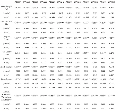
Table 5, shows the compilation of correlation coefficients with their corres-ponding t-statistics and p-value over the period of 2005 to 2016. Proceeding by variable, the compilation table reveals a strong but negative correlation between the container throughput and quay length at 5% of significance for years 2010 and 2011. Any other correlation coefficient with respect to container throughput and quay length within the time frame of our study, are not statistically signifi-cant. The terminal area, on the other hand, is highly correlated with the output variable from the year 2005 to 2011, and the year 2015, at 1% of significance. A positive correlation for the years 2012, 2014 and 2016 is also noticed at a 5% of significance. The container throughput is positively correlated to the number of quayside cranes from 2005 to 2012 at 1% significance, while positively correlated at a 5% significance for the years 2013, 2015 and 2016. The container throughput is highly correlated to the number of yard gantry cranes at 1% significance for the year 2013 while showing a 5% significance for the years 2012 and 2015.

The number of reach stackers is positively correlated to container throughput from the year 2005 to 2011 at a 1% significance and is still correlated at a 5% significance for the year 2012. Other correlation coefficients with respect to con-tainer throughput and the number of reach stackers are not significant. The draught is statistically significant at 1% from 2012 to 2014, implying a high cor-relation with the container throughput. A 5% significance for the years 2010 and 2011 is noticed. Other years within the study time period shown to be not con-clusive. The container throughput and the annual container throughput limit are positive and highly correlated at 1% of significance over all the years of the study period. A significance of 1%, shows a strong predictive relationship between the variables.

(14)

[image:14.595.61.534.89.546.2]

DOI: 10.4236/jtts.2019.93018 300 Journal of Transportation Technologies Table 5. Compilation table of container throughput vs. input variables over time.

CT2005 CT2006 CT2007 CT2008 CT2009 CT2010 CT2011 CT2012 CT2013 CT2014 CT2015 CT2016 Quay Length

(m) −0.326 −0.506* −0.552* −0.440 −0.265 −0.668** −0.696** −0.032 −0.270 −0.181 0.535* 0.366 (p-value) −0.301 −0.093 −0.062 −0.152 −0.406 −0.017 −0.012 −0.921 −0.397 −0.573 0.073 0.242 (t-stat) −1.092 −1.857 −2.098 −1.551 −0.868 −2.843 −3.072 −0.102 −0.885 −0.582 2.004 1.244 Terminal Area

(Ha) 0.937*** 0.875*** 0.836*** 0.911*** 0.860*** 0.858*** 0.780*** 0.687** 0.566* 0.640** 0.745*** 0.661** (p-value) 0.000 0.000 0.001 0.000 0.000 0.000 0.003 0.013 0.055 0.025 0.005 0.019

(t-stat) 8.531 5.742 4.819 6.999 5.339 5.298 3.952 2.996 2.173 2.635 3.535 2.787 Quayside

Cranes 0.867*** 0.960*** 0.970*** 0.932*** 0.853*** 0.996*** 0.984*** 0.901*** 0.681** 0.020 0.702** 0.627** (p-value) 0.000 0.000 0.000 0.000 0.000 0.000 0.000 0.000 0.015 0.951 0.011 0.029

(t-stat) 5.508 10.986 12.792 8.177 5.169 35.542 17.741 6.578 2.946 0.062 3.119 2.550 Yard Gantry

Cranes 0.518* 0.235 0.139 0.342 0.414 0.109 −0.016 0.585** 0.797*** 0.516* 0.634** 0.470 (p-value) 0.084 0.461 0.667 0.276 0.181 0.737 −0.962 0.046 0.002 0.085 0.027 0.123 (t-stat) 1.916 0.766 0.443 1.151 1.438 0.346 −0.049 2.283 4.182 1.909 2.593 1.683 Reach Stackers 0.859*** 0.970*** 0.985*** 0.938*** 0.911*** 0.959*** 0.964*** 0.639** 0.443 −0.438 0.313 0.152 (p-value) 0.000 0.000 0.000 0.000 0.000 0.000 0.000 0.025 0.149 −0.154 0.322 0.637 (t-stat) 5.321 12.687 18.688 8.558 6.988 10.779 11.568 2.634 1.565 −1.543 1.042 0.487 Draught (m) −0.536* −0.488 −0.467 −0.470 −0.488 −0.693** −0.667** −0.709*** −0.936*** −0.911*** −0.408 −0.482

(p-value) −0.072 −0.107 −0.126 −0.123 −0.107 −0.012 −0.018 −0.010 0.000 0.000 −0.188 −0.112 (t-stat) −2.009 −1.769 −1.672 −1.683 −1.769 −3.047 −2.837 −3.180 −8.453 −6.998 −1.413 −1.740 Annual

Container Throughput Limit (TEU)

0.986*** 0.929*** 0.890*** 0.965*** 0.942*** 0.884*** 0.811*** 0.981*** 0.945*** 0.964*** 0.863*** 0.858***

(p-value) 0.000 0.000 0.000 0.000 0.000 0.000 0.001 0.000 0.000 0.000 0.000 0.000 (t-stat) 19.201 7.989 6.195 11.643 8.935 5.987 4.390 16.110 9.210 11.557 5.412 5.286

***, **, *imply significance of 1, 5, and 10% respectively. Source: Processed by the Author.

and annual container throughput limit. The study here aims at identifying va-riables that in terms of efficiency and performance, drive and predict these ports container throughput. Having a pre-knowledge on these input variables is essen-tial for container ports activities. Analyzing the variables on a yearly basis, re-vealed the terminal area, the quayside cranes and annual container throughput limit were the only significant variables correlated to the container throughput in the year 2016. However, if compared to the base year 2005, there four out of seven input variables were positive and statistically significant at 1%.

(15)

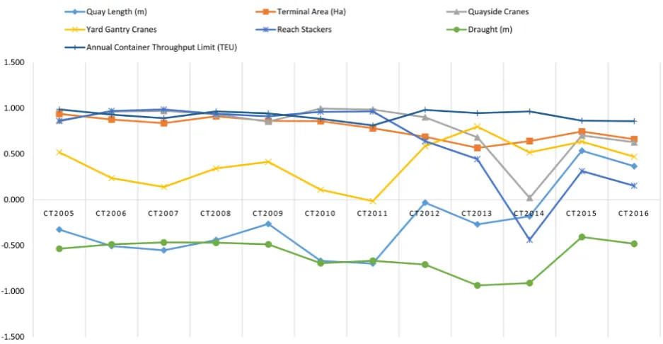
limit, the quayside cranes, the terminal area, and the reach stackers. The quay length correlation to the container throughput also tended to zero from 2011 to 2012 and then from 2013 to 2014. These shifts of the mentioned variables were largely due to the insecurity from terrorism threats which prevailed in West Africa at that time. The reach stackers, the quay length, the quayside cranes and the yard gantry cranes quayside cranes and terminal area moved toward a much better correlation with the container throughput from 2014 to 2015. All the va-riables experienced a downward slope in 2016 from the previous year, with the exception of draught inversely correlated to the container throughput.

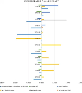
A close look at the compiled p-value chart in Figure 2 gives a clear overview of the uncorrelated variables across years. These are the quay length, the yard gantry cranes, and the draught. Throughout the last four years of the study, reach stackers showed no significant correlation in explaining variation in the container throughput. Hence, the reliable and statistically significant in explain-ing changes in the container throughput, for the time period of the research, are the terminal area, quayside cranes, reach stackers, and the annual container throughput limit.

[image:15.595.65.534.464.707.2]

The frequency of very strong correlation, have been noticed between the con-tainer throughput and the terminal area, the quayside cranes, the reach stackers, and annual container throughput limit. With minor variations to be considered, five variables were found to reveal a long-run positive sign with the output vari-able; these were the annual container throughput limit, reach stackers, yard gan-try cranes, quayside cranes, terminal area. On the other hand, the remaining two variables are exhibiting a negative long-run relationship with container throughput, these are quay length and draught.

(16)

DOI: 10.4236/jtts.2019.93018 302 Journal of Transportation Technologies Figure 2. Uncorrelated variable probability value chart, from year 2005-2016. Source: Processed by the Author.

6. Conclusion

[image:16.595.215.531.73.429.2]

(17)

10.47% for instance, if the quay length is well utilized (meaning that more con-tainership is berthing at the ports), then a positive relationship could be estab-lished with the container throughput throughout time (implying an infrastruc-ture project development as throughput increases with time). On the opposite side, a negative but significant correlation in this case, can express that the ports are too small regarding the activities they perform. Outcome highlights that three ports (Tema, Lagos and Lomé) exhibited constant returns to scale (CRS). In addition, other two ports (Abidjan and Cotonou) are operating at increasing returns to scale. Due to their small size of production, they should enhance their efficiency by selecting a scaling up strategy that will increase their scale of opera-tions. Consequently, the study found that the container throughput at these five ports was more dependent on the terminal area, the quayside cranes, reach stackers and the annual container throughput limit.

Conflicts of Interest

The authors declare no conflicts of interest regarding the publication of this paper.

References

[1] Adam, S. (1982) The Wealth of Nations Books I-III. Penguin Classics, London. [2] Talley, W.K. (2009) Port Economics. Routledge, London and New York.

https://doi.org/10.4324/9780203880067

[3] Slack, B. (1985) Containerization, Inter-Port Competition and Port Selection. Mari-time Policy and Management, 12, 293-303.

https://doi.org/10.1080/03088838500000043

[4] Hayuth, Y. (1988) Rationalization and Deconcentration of the U.S. Container Port System. The Professional Geographer, 40, 279-288.

https://doi.org/10.1111/j.0033-0124.1988.00279.x

[5] The World Bank (2017) World Bank Data. https://data.worldbank.org

[6] Statista (2017) Container Shipping—Statistics & Facts. Transportation & Logistics, Water Transport. https://www.statista.com/topics/1367/container-shipping [7] Rodrigue, J.-P. (2017) The Geography of Transport Systems. Routledge Taylor and

Francis Group, New York.

[8] van Dyck, G.K. (2016) An Empirical Assessment of Inter-Port Competition in West Africa towards Hub Port Selection. Doctoral Dissertation, Shanghai Maritime Uni-versity, Transport Engineering Economics and Management, Shanghai.

[9] Kalgora, B. (2019) Strategic Container Ports Competitiveness Analysis in West Africa Using Data Envelopment Analysis (DEA) Model. Open Journal of Business and Management, 7, 680-692.https://doi.org/10.4236/ojbm.2019.72046

[10] Van de Voorde, E. and Winkelmans, W. (2002) A General Introduction to Port Competition and Management. In: Huybrechts, M. and Meers, H., Eds., Port Com-petitiveness: An Economic and Legal Analysis of the Factors Determining the Competitiveness of Seaports, The National Academies of Sciences, Engineering, and Medicine, Washington DC, 1-16.

(18)

http://www.mapsofworld.com/africa/regions/western-africa-map.html

[12] ECOWAS (2015) Member States. Economic Community of West African States.

http://www.ecowas.int/member-states

[13] AFDB (2015) Economic Transformation. African Development Bank, Abidjan. http://www.afdb.org/en/blogs/measuring-the-pulse-of-economic-transformation-in

-west-africa

[14] Kalgora, B. (2019) Intermodal Terminal Localisation Using a Linear Programming Approach: The Case Study of Togo and West African Landlocked Countries. Jour-nal of Transportation Technologies, 9, 215-231.

https://doi.org/10.4236/jtts.2019.92014

[15] van Dyck, G.K. (2015) The Drive for a Regional Hub Port for West Africa: General Requirements and Capacity Forecast. International Journal of Business and Eco-nomics Research, 4, 36-44.https://doi.org/10.11648/j.ijber.20150402.13

[16] Monteiro, M. (2014) Productivity in the Container Port Business—Case Study of the Mediterranean Range. University of Antwerp, Antwerp.

[17] Notteboom, T. and Rodrigue, J. (2008) Containerisation, Box Logistics and Supply Chains: The Integration of Ports in Liner Shipping Networks. Maritime Economics and Logistics, 10, 1152-1174.https://doi.org/10.1057/palgrave.mel.9100196

[18] Wu, Y.C.J. and Goh, M. (2010) Container Port Efficiency in Emerging and More Advanced Markets. Transportation Research Part E, 46, 1030-1042.

https://doi.org/10.1016/j.tre.2010.01.002

[19] Demirel, B., Cullinane, K. and Haralambides, H. (2012) Container Terminal Effi-ciency and Private Sector Participation. In: Talley, W.K., Ed., The Blackwell Com-panion to Maritime Economics, Blackwell Publishing Ltd., Hoboken, 571-598.

https://doi.org/10.1002/9781444345667.ch28

[20] Liu, Q. (2010) Efficiency Analysis of Container Ports and Terminals. PHD Thesis, Centre for Transport Studies, University College of London, London.

[21] Porter, M. (1990) The Competitive Advantage of Nations. Harvard Business Re-view, 68, 73-93.https://doi.org/10.1007/978-1-349-11336-1

[22] van Dyck, G.K. (2015) Assessment of Port Efficiency in West Africa Using Data Envelopment Analysis (DEA). American Journal of Industrial and Business Man-agement, 5, 208-218. https://doi.org/10.4236/ajibm.2015.54023

[23] Padilla, M. and Eguia, R. (2010) Relative Efficiency of Seaports in Mindanao. 11th National Convention on Statistics (NCS), Manila, 11-13 October 2010, 1-15. [24] Fried, H.O., Lovell, C.A.K. and Schmidt, S.S. (2008) The Measurement of

Produc-tive Efficiency and Productivity Growth. Oxford University Press, New York.

https://doi.org/10.1093/acprof:oso/9780195183528.001.0001

[25] Anguibi, C.F.C. (2015) Analyzing the Operational Efficiency of Container Ports in Sub-Saharan Africa. Open Journal of Social Sciences, 3, 10-17.

https://doi.org/10.4236/jss.2015.310002

[26] Coelli, T. (1996) A Guide to FRONTIER Version 4.1: A Computer Program for Frontier Production Function Estimation. University of New England Department of Econometrics, CEPA Working Paper 96/07, Armidale.

[27] Cullinane, K.W.F., Song, D.W. and Ji, P. (2006) The Technical Efficiency of Con-tainer Ports; Comparing Data Envelopment Analysis and Stochastic Frontier Anal-ysis. Transportation Research Part A: Policy and Practice, 40, 354-374.

https://doi.org/10.1016/j.tra.2005.07.003

(19)

Effi-DOI: 10.4236/jtts.2019.93018 305 Journal of Transportation Technologies ciency: A Comparative Study of DEA and FDH Approaches. Journal of the Eastern Asia Society for Transportation Studies, 5, 698-713.

[29] Martinez-Budria, E., Diaz-Armas, R., Navarro-Ibanez, M. and Ravelo-Mesa, T. (1999) A Study of the Efficiency of Spanish Port Authorities Using Data Envelop-ment Analysis. International Journal of Transport Economics, 26, 237-253. [30] Tongzon, J. (2001) Efficiency Measurement of Selected Australian and Other

Inter-national Ports Using Data Envelopment Analysis. Transportation Research Part A:

Policy and Practice, 35, 113-128.

https://doi.org/10.1016/S0965-8564(99)00049-X

[31] Degbe, S.A. (2017) An Empirical Study on Transit Traffic via West African Corri-dors: Case Study of Lomé-Ouagadougou. Master Thesis Dissertation, Shanghai Ma-ritime University, Transport Planning and Management, Shanghai.

[32] Cullinane, K.P., Wang, T.F. and Cullinane, S.L. (2004) Container Terminal Devel-opment in Mainland China and Its Impact on the Competitiveness of the Port of Hong Kong. Transport Reviews, 24, 33-56.

https://doi.org/10.1080/0144164032000122334

[33] Min, H. and Park, B. (2005) Evaluating the Inter-Temporal Efficiency Trends of In-ternational Container Terminals Using Data Envelopment Analysis. International Journal of Integrated Supply Management, 1, 258-277.

https://doi.org/10.1504/IJISM.2005.005950

[34] Al-Eraqi, A.S., Barros, C.P., Mustaffa, A. and Khader, A.T. (2008) Efficiency of Middle Eastern and East African Seaports: Application of DEA Using Window Analysis. European Journal of Scientific Research, 23, 597-612.

[35] Ancor, S.-A., Javier, M.S., Tomás, S. and Lourdes, T. (2016) When It Comes to Container Port Efficiency, Are All Developing Regions Equal? Transportation Re-search Part A, 86, 56-77.https://doi.org/10.1016/j.tra.2016.01.018

[36] Roll, Y. and Hayuth, Y. (2006) Port Performance Comparison Applying Data Enve-lopment Analysis (DEA). Maritime Policy & Management, 20, 153-161.

https://doi.org/10.1080/03088839300000025

[37] Cullinane, K.P. and Wang, T.-F. (2006) The Efficiency of European Container Ports: A Cross-Sectional Data Envelopment Analysis. International Journal of Lo-gistics: Research and Applications, 9, 19-31.

https://doi.org/10.1080/13675560500322417

[38] Munisamy, S. and Singh, G. (2011) Benchmarking the Efficiency of Asian Container Ports. African Journal of Business Management, 5, 1397-1407.

[39] PMAWCA (2017). http://www.agpaoc-pmawca.org

[40] Sherman, H.D. and Zhu, J. (2006) Service Productivity Management Improving Service Performance Using Data Envelopment Analysis (DEA).

[41] Charnes, A., Cooper, W.W. and Rhodes, E. (1978) Measuring the Efficiency of De-cision Making Units. European Journal of Operational Research, 2, 429-444.

https://doi.org/10.1016/0377-2217(78)90138-8

[42] Banker, R.D., Charnes, A. and Cooper, W.W. (1984) Some Models for Estimating Technical and Scale Inefficiencies in Data Envelopment Analysis. Management Science, 30, 1078-1092.https://doi.org/10.1287/mnsc.30.9.1078

(20)

[image:20.595.60.535.96.736.2]

Appendix

Table A1. Data inputs and output variables.

Port Variables 2005 2006 2007 2008 2009 2010 2011 2012 2013 2014 2015 2016

Port of Abidjan

Container

Throughput 710,000 507,119 469,277 652,358 610,185 561,535 546,417 633,917 745,102 783,102 835,312 705,000

Total Quay

Length 640 640 640 640 640 640 640 1000 1000 1000 1000 1000

Terminal

Area 34 34 34 34 34 34 34 34 34 34 34 34

Number of Quayside

Cranes 5 5 5 5 5 5 5 7 7 7 7 7

Number of Yard Gantry Cranes

12 12 12 12 12 12 12 16 16 16 16 16

Number of Reach

Stackers 10 10 10 10 10 10 10 16 16 16 16 16

Draught 11.5 11.5 11.5 11.5 11.5 11.5 11.5 11.5 11.5 11.5 11.5 11.5

Limit

1,200,000 1,200,000 1,200,000 1,200,000 1,200,000 1,200,000 1,200,000 1,200,000 1,200,000 1,200,000 1,500,000 1,500,000

Port of Cotonou

Container

Throughput 158,201 145,230 163,240 193,745 272,820 316,744 334,798 348,190 388,341 408,146 472,154 333,000 Total

Quay

Length 400 400 400 400 400 400 400 600 600 600 600 600

Terminal

Area 14.5 14.5 14.5 14.5 14.5 14.5 14.5 14 14 14 14 14

Number of Quayside

Cranes 4 4 4 4 4 4 4 6 6 6 6 6

5 5 5 5 5 5 5 10 10 10 10 10

Number of Reach

Stackers 8 8 8 8 8 8 8 15 15 15 15 15

Draught 11.7 11.7 11.7 11.7 11.7 13.5 13.5 13.5 13.5 13.5 13.5 13.5

Limit

(21)

DOI: 10.4236/jtts.2019.93018 307 Journal of Transportation Technologies Continued

Port of Lagos

Container

Throughput 870,015 875,020 903,530 947,400 710,800 1,128,171 1,413,273 1,623,141 1,010,836 1,062,389 1,156,287 1,335,470 Total

Quay

Length 120 120 120 120 120 120 120 1210 1210 1210 1210 1210

Terminal

Area 45 45 45 45 45 45 45 42 42 42 42 42

Number of Quayside

Cranes 8 8 8 8 8 8 8 12 12 12 12 12

5 5 5 5 5 5 5 14 14 14 14 14

Number of Reach

Stackers 13 13 13 13 13 13 13 17 17 17 17 17

Draught 11.5 11.5 11.5 11.5 11.5 11.5 11.5 11.5 11.5 11.5 11.5 11.5

Limit

1,500,000 1,500,000 1,500,000 1,500,000 1,500,000 1,500,000 1,500,000 2,000,000 2,000,000 2,000,000 2,000,000 2,000,000

Port of Lome

Container

Throughput 204,614 215,898 237,891 296,109 354,480 339,853 352,695 288,481 311,470 380,798 905,700 821,639

Total Quay

Length 480 480 480 480 480 480 480 1752 1752 1752 1752 1752

Terminal

Area 12 12 12 12 12 12 12 23 23 23 23 23

Number of Quayside

Cranes 4 4 4 4 4 4 4 8 8 14 14 14

Number of Yard Gantry

Cranes 2 2 2 2 2 2 2 6 6 13 13 13

Number of Reach

Stackers 9 9 9 9 9 9 9 15 15 23 23 23

Draught 14.5 14.5 14.5 14.5 14.5 14.5 14.5 14.5 14.5 14.5 14.5 14.5

Limit

450,000 450,000 450,000 450,000 450,000 450,000 450,000 550,000 550,000 550,000 1,000,000 1,000,000

Port of

Tema Throughput 442,082 476,451 513,204 518,336 525,694 590,147 756,899 824,238 841,989 833,771 856,911 925,964 Container

Total Quay

(22)

DOI: 10.4236/jtts.2019.93018 308 Journal of Transportation Technologies Continued

Termina

Area 14 14 14 14 14 14 14 14 14 14 14 14

Number of Quayside

Cranes 5 5 5 5 5 5 5 8 8 8 8 8

3 3 3 3 3 3 3 12 12 12 12 12

Number of Reach

Stackers 11 11 11 11 11 11 11 14 14 14 14 14

Draught 11.5 11.5 11.5 11.5 11.5 11.5 11.5 11.5 11.5 11.5 11.5 11.5

Limit

650,000 650,000 650,000 650,000 650,000 650,000 650,000 1,200,000 1,200,000 1,200,000 1,200,000 1,200,000