On the Global Convergence of the PERRY SHANNO Method for Nonconvex Unconstrained Optimization Problems

(1)

doi:10.4236/am.2011.23037 Published Online March 2011 (http://www.scirp.org/journal/am)

On the Global Convergence of the PERRY-SHANNO

Method for Nonconvex Unconstrained

Optimization Problems*

Linghua Huang1, Qingjun Wu2, Gonglin Yuan3 1

Department of Mathematics and Statistics, Guangxi University of Finance and Economics, Nanning, China

2

Department of Mathematics and Computer Science, Yulin Normal University, Yulin,China

3

Department of Mathematics and Information Science, Guangxi University, Nanning, China E-mail: linghuahuang@163.com, wqj600@yahoo.com.cn, [email protected] Received November 15, 2010; revised January 12, 2011; accepted January 16, 2011

Abstract

In this paper, we prove the global convergence of the Perry-Shanno’s memoryless quasi-Newton (PSMQN) method with a new inexact line search when applied to nonconvex unconstrained minimization problems. Preliminary numerical results show that the PSMQN with the particularly line search conditions are very promising.

Keywords: Unconstrained Optimization, Nonconvex Optimization, Global Convergence

1. Introduction

We consider the unconstrained optimization problem:

 





min f x xRn , (1.1) where f R: n Ris continuously differentiable. Perry and Shanno’s memoryless quasi-Newton method is often

used to solve the problem (1.1) when

n

is large. The

PSMQN method was originated from the works of Perry (1977 [1]) and Shanno (1978 [2]), and subsequently de-veloped and analyzed by many authors. Perry and Shan-no’s memoryless method is an iterative algorithm of the form

1

k k k k

x_ x  d , (1.2) where k is a steplength, anddkis a search direction

which given by the following formula:

1 1

d  g , (1.3)

1 1

1 2 1 2

1 2

2

, 1

T T T

k k k k k k

k k T k

k k

T k k

k k

y s y g s g

d g s

y s

y y

s g

y k y

 



 

 

   

 

 

 

(1.4)

wheresk xk1x yk, k gk1gkand gj denotes the

gradient of f at xj. If we denote

2 2

1 2

T

k k k k T

k T T _T k k

k k k k k k k

y y y y

B I s s

y s y s s y s

    (1.5)

and

1

1 1

k k

H _ B_ ,

then





1 2 2

1 2

T T

k k k k

k T k k k k

k k

y s s s

H I s y y s

y s

y y

     . (1.6)

By (1.4) and (1.5), we can rewrite dk1 as

1 1 1

k k k

d  H g .

In practical testing, it is shown that the memoryless method is much more superior to the conjugate gradient methods, and in theoretic analysis, Perry and Shanno had proved that this method will be convergent for uniform convex function with Armijor or Wolfe line search. Shanno pointed out that this method will be convergent for convex function if the Wolfe line search is used. De-spite of many efforts has been put to its convergence behavior, the global convergence of the PSMQN method is still open for the case of f is not a convex function. Recently, Han, Liu and Yin [3] proved the global con-vergence of the PSMQN method for nonconvex function under the following condition

lim _k 0

k s  .

(2)

The purpose of this paper is to study the global con-vergence behavior of PSMQN method by introducing a new line search conditions. The line search strategy used in this paper is as follows: find tk satisfying





 





2 4

1

min ,

T

k k k k k k k k k k

f x t d  f x t g d   g  t d

(1.7) and





T _T

k k k k k k

g x t d d g d , (1.8) where1

 

0,1 s a small scalar and 



1,



is a

large scalar. It is clear that (1.7) and (1.8) are a modifica-tion of the weak Wolfe-Powell (MWWP) line search conditions.

This paper is organized as follows. In Section 2, we present the PSMQN with the new line search MWWP. In Section 3, we establish the global convergence of the proposed method. The preliminary numerical results are contained in Section 4.

2. Algorithm

By combining the PSMQN and the MWWP, we can ob-tain a modified Perry-Shanno’s memoryless quasi-Newton method as follows:

Algorithm 1 (A Modified PSMQN method: MPS- MQN)

Step 0: Given 1

n

x R , set d1 g k1, 1. If g10,

then stop.

Step 1: Find a t_k 0 satisfying MWWP.

Step 2: Let xk1xkt dk k and gk1g x



k1



. If

1 0

k

g _  , then stop.

Step 3: Generate dk1 by the PSMQN formula (1.4).

Step 4: Set k: k 1, go to Step 1.

3. Global Convergence

In order to prove the global convergence of Algorithm 1, we will impose the following two assumptions, which have been used often in the literature to analyze the global convergence of conjugate gradient and quasi-Newton methods with inexact line searches.

Assumption A. The level set

 



1



n

x R f x f x

   

is bounded.

Assumption B. There exists a constant

L

such that for anyx y,  ,

 

g x g y L xy . (3.1)

Since



f x

 

k



is a decreasing sequence, it is clear that

the sequence

 

x_k generated by Algorithm 1 is contained

in, and there exists a constant f, such that

 

lim _k

k f x f



  . (3.2)

Lemma 3.1 Suppose that Assumption A holds and there exists a positive constant  such that

k

g . (3.3) then,

2

lim k k 0

kt d  (3.4)

and

2

lim k k 0

kt d  . (3.5)

Proof. From (3.2), we have

 











 





 









 

1 1

1

lim

.

N

k k k k

N

k k

k N

f x f x f x f x

f x f x f x f



 _ 

 

 



  

 



thus

 







1



1

,

k k

k

f x f x



 

  



which combining with





 





₂ 4

1

min ,

T

k k k k k k k k k k

f x t d f x t g d   g  t d and (3.3), yields

4 2

1 k k k

t d





 



, (3.6)

and

1 T k k k k

t g d





  



. (3.7)

therefore, (3.4) and (3.5) hold.

The property (3.4) is very important for proving the global convergence of Algorithm 1, and it is not known yet for us whether (3.4) holds for other types line search (for example, the weak Wolfe-Powell conditions or the strong Wolfe-Powell conditions).

By using (3.4) and the result given in [3], we can de-duce that Algorithm 1 is convergent globally. In the fol-lowing, we give a direct proof for the global convergence of Algorithm 1.

Lemma 3.2 Assume thatBkis a positive definite

ma-trix. Then

 

2

k

r k T

k k k g

T B

g H g  . (3.8)

Proof. Omitted.

Lemma 3.3 Supposed that Assumption A and B hold, and xk is generated by Algorithm 1.Then there exists a

(3)

1 k k i t ck  



. (3.9)

Proof. By (1.5) and (1.6), we have



1



2

k

r k T

k k y

T B n

y s

  , (3.10)

and



1

 

2



2 2 2

T

k k k

r k T

k k k

y s s

T H n

y s y

    . (3.11)

From



y sTk k



2 sk 2 yk 2, we obtain



1

 

2



2 2 2

T

k k k

r k T

k k k

y s s

T H n

y s y

    . (3.12)

Using (1.8) and (3.12), we have



1



2

1

k k k

r k T

k k k t H g n

T H

g H g 

  _ . (3.13)

By using the positive definiteness of Hk, we have

 

2

k k

r k T

k k k H g

T H

g H g  , (3.14)

from which we can deduce that



1



 

1

k

r k r k

i n

T H T H t







 

  _ 

 



. (3.15)

By the Assumption B, (3.10) and (1.8), we get









 

2 1 2 2 2 2 2 1 1 1 1 , k

r k T

k k k T k k k k k T

k k k

k k k T

k k k

k r k y

T B n

y s s nL g s H g nL t

g H g

H g c t

g H g

c t T H            , where 2 1 1 nL c  

 . Combining with (3.15) yields



1



1 1

 

1

k _k

r k k r k

i n

T B c t T H t

       _ _   



.

Adding above inequality to (3.15), we obtain













 





1

1 1 1

1

1 .

1

k

r k r k k r k

i

c n

T B T H T H t

n           _  _   



Now, if we denote the eigenvalues of Bk by

1, 2, ,

k k kn

h h  h , then the eigenvalues of

H

_k are

1 2

1 1 1

, , ,

k k kn

h h  h , so we have



1





1



1

1 2

n

r k r k ki

i ki

T B T H h n

h        _  _  



.

Thus we have

 





1 ₁ 1 2 1 1 1 k k k i r n t c n T H n          _    _     



.

Hence there exists a positive constant

c

such that

1 k k k i t c  



. Therefore 1 k k i t ck  



.

Theorem 3.1 Supposed that Assumption A and B hold, and

x

k is generated by Algorithm 1.Then

lim inf _k 0

k g  . (3.16) Proof. Suppose that the conclusion doesn’t hold, i.e., there exists a positive constant



such that

k

g .

From (3.3), (3.10) and Lemma 3.3, we have





















 





 

2 1 2 2 2 2 2 2 2 2 2 2 2 2 2 1 2 1 1 2 2 1 1 1 1 1 1 1 , k

r k T

k k

k T

k k k k

k k T

k k k k k

k k

T k k k k

k

r k k

k

k k

r i i

i i

k k

r i i

i y

T B n

y s y n

t g H g

y g

n

t g g H g

nL s g

t g H g nL s

T B t

nL

T B s t

c T B t d

                             _ _ _             



 where





2 2 2 1 nL c   

(4)

there exists a positive constant

k

0 such that

2 2

1

i i t d

c

 for all ik0.

Therefore



    

 





0

0 0

0

0 0

2 2

1 2 2 1

1 1

2

2 1 3

1

3

1 3

1

.

k k

k k k

r k r i i i i

i i k

k k

r i i

i

k i i

T B c c T B t d t d

c T B t d c

c k

c t c

 

  









 

 







Hence from the above inequality and Lemma 3.2 and Lemma 3.3, we have

 

3

1 1

1 3

2 1 3

2 1

.

k k

k

i i k i r k

T k k k k

i _k

T k k k k i

t c t

c T B

t

c t g H g

c _g

c

t g H g c

 

 _ 



 



 

  

 

 



  



Therefore

1 k i

t





 



,

which contradicts to Lemma 3.3. Thus (3.16) holds.

Remark: In this remark, we give a cautious update of Perry-Shanoo’s Memoryless quasi-Newton method (CP- SMQN), we do not discuss the global convergence here. We let it to be a topic of further research.

Algorithm 2: (CPSMQN method)

Step 0: Given 1

n

x R , set d1 g k1, 1. If g10,

then stop.

Step 1: Find a tk 0satisfying WWP.

Step 2: Let xk1xkt dk k and gk1g x



k1



. If

1 0

k

g  , then stop.

Step 3: Choose Bk1 by the following equation and

Generate dk1,

2 2

1

if ,

else

T T

k k k k T k k

k k

T T T

k k k k k k k k k

k

y y y y g s

I s s m

B y s y s s y s s

B



 _

   

   

(3.17) where m is a positive constant.

4. Numerical Experiments

In this section, we report the numerical results for

PSM-QN, MPSMQN and CPSMQN method. The problems that we tested are from [4]. For each test problem, the termination condition is

5

10 )

(

x

k





g

.

We will test the following three methods:

•PSMQN: the Perry-Shanno’s Memoryless quasi-

Newton method with the WWP, where  0.1 and

0.9

  ;

•MPSMQN: Algorithm 1 with  0.1,  0.9,

16 1 10

 _ 

and 10;

• CPSMQN: Algorithm 2 with  0.1, 0.9 and

18

10

m  .

In order to rank the iterative numerical methods, one can compute the total number of function and gradient evaluations by the formula

,

total

N NF m NG (4.1)

where NF NG, denote the number of function

evalua-tions and gradient evaluaevalua-tions, respectively, and m is some integer. According to the results on automatic dif-ferentiation ([5] and [6]), the value of m can be set to

5

m . That is to say, one gradient evaluation is equiva-lent to m number of function evaluations if automatic differentiation is used.

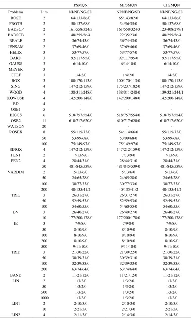
Tables 1 shows the computation results, where the co- lumns have the following meanings:

Problem: the name of the test problem in MATLAB; Dim: the dimension of the problem;

NI: the number of iterations;

NF: the number of function evaluations; NG: the number of gradient evaluations;

SD: the number of iterations for which the steepest descent direction used;

In this part, we compare the PSMQN, MPSMQN and

CPSMQN method as follows: for each testing examplei,

compute the total numbers of function evaluations and gradient evaluations required by the evaluated method

 





j EM j and the PSMQN method by the formula (4.1), and denote them by N_{total i EM j}_,_ _{ }_andNtotal i PSMQN,_ _;

then calculate the ratio

 





  

 

,

, total i EM j i

total i PSMQN

N r EM j

N

 . (4.2)

If EM j

 

0 does not work for example

i

0, we replace

the _ _{ }_

0 0

,

total i EM j

N by a positive constant



which define

as follows

 



, 1



max N_{total i EM j} : ,i j S

   ,

where

 



1 , :

(5)

[image:5.595.109.487.93.722.2]

Table 1. Test results for PSMQN/MPSMQN/CPSMQN.

PSMQN MPSMQN CPSMQN

Problems Dim NI/NF/NG/SD NI/NF/NG/SD NI/NF/NG/SD ROSE

FROTH BADSCP BADSCB BEALE JENSAM

HELIX BARD GAUSS MEYER GULF

BOX SING WOOD KOWOSB

BD OSB1 BIGGS

OSB2 WATSON

ROSEX

SINGX PEN1 PEN2

VARDIM

TRIG

BV

IE

TRID

BAND LIN

LIN1

LIN2

2 2 2 2 2 2 3 3 3 3 3 3 4 4 4 4 5 6 11 20 8 50 100

4 2 4 50

2 50 100 200 3 50 100

3 10

3 50 100 200 500 3 50 100 200 2 2 50 500 1000

2 10

4

64/133/86/0 50/137/68/0 161/558/324/3

48/255/56/4 36/74/43/0 37/69/46/0 53/77/57/0 92/117/95/0

6/14/10/0 - 1/4/2/0 100/170/113/0 147/212/159/0 138/311/248/0 142/200/148/0

- - 518/757/554/0 610/717/620/0

- 55/115/73/0

53/99/68/0 75/149/97/0 147/212/159/0

7/13/9/0 28/44/31/0 481/845/539/0

5/13/6/0 24/65/28/0 30/77/33/0 40/135/41/2

26/31/27/0 52/59/53/0 54/60/55/0 26/40/27/0 177/200/178/0

7/9/8/0 8/10/9/0 8/10/9/0 8/10/9/0 9/11/10/0 21/30/22/0 30/39/31/0 32/39/33/0 63/74/64/0 11/21/12/0 1/3/2/0 1/3/2/0 1/3/2/0 1/3/2/0 2/10/3/0 2/21/3/0 2/11/3/0

65/143/82/0 34/56/35/0 161/558/324/3

22/35/23/0 36/74/43/0 37/69/46/0 53/77/57/0 92/117/95/0

6/14/10/0 - 1/4/2/0 100/170/113/0 175/237/182/0 138/311/248/0 142/200/148/0

- - 518/757/554/0 610/717/620/0

- 54/114/66/0

53/99/68/0 75/149/97/0 147/212/159/0

7/13/9/0 28/44/31/0 481/845/539/0

5/13/6/0 24/65/28/0 30/77/33/0 40/135/41/2

26/31/27/0 52/59/53/0 54/60/55/0 26/40/27/0 177/200/178/0

7/9/8/0 8/10/9/0 8/10/9/0 8/10/9/0 9/11/10/0 21/30/22/0 30/39/31/0 32/39/33/0 63/74/64/0 11/21/12/0 1/3/2/0 1/3/2/0 1/3/2/0 1/3/2/0 2/10/3/0 2/21/3/0 2/14/3/0

64/133/86/0 50/137/68/0 123/408/279/1

48/255/56/4 36/74/43/0 37/69/46/0 53/77/57/0 92/117/95/0

6/14/10/0 - 1/4/2/0 100/170/113/0 147/212/159/0 139/321/244/1 142/200/148/0

- - 518/757/554/0 610/717/620/0

- 55/115/73/0

53/99/68/0 75/149/97/0 147/212/159/0

7/13/9/0 28/44/31/0 481/845/539/0

5/13/6/0 24/65/28/0 30/77/33/0 40/135/41/2

26/31/27/0 52/59/53/0 54/60/55/0 26/40/27/0 177/200/178/0

(6)

Table 2. Relative efficiency of PSMQN, MPSMQN and CPSMQN.

PSMQN MPSMQN CPSMQN

1 0.9752 0.9963

The geometric mean of these ratios for method EM( j)

over all the test problems is defined by

 





i



 



1S

i S

r EM j r EM j



 

  





 , (4.3)

where S denotes the set of the test problems and S

the number of elements in S . One advantage of the above rule is that, the comparison is relative and hence does not be dominated by a few problems for which the me-thod requires a great deal of function evaluations and gradient functions.

From Table 2, we observe that the average

perfor-mances of the Algorithm 1 are the best among the three methods, and the average performances of the Algorithm 2 are little better than the PSMQN method. Therefore, the Algorithm 1 is the best method among the three me-thods given in this paper from both theory and the com-putational point of view.

5. References

[1] J. M. Perry, “A Class of Conjugate Algorithms with a Two Step Variable Metric Memory,” Discussion paper 269, Northwestern University, 1977.

[2] D. F. Shanno, “On the Convergence of a New Conjugate Gradient Algorithm,” SIAM Journal on Numerical Anal-ysis, Vol. 15, No. 6, 1978, pp. 1247-1257.

doi:10.1137/0715085

[3] J. Y. Han, G. H. Liu and H. X. Yin, “Convergence of Perry and Shanno’s Memoryless Quasi-Newton Method of Nonconvex Optimization Problems,” On Transactions, Vol. 1, No. 3, 1997, pp. 22-28.

[4] J. J. More, B. S. Garbow and K. E. Hillstrome, “Testing Unconstrained Optimization Software,” ACM Transac-tions on Mathematical Software, Vol. 7, No. 1, 1981, pp. 17-41. doi:10.1145/355934.355936

[5] A. Griewank, “On Automatic Differentiation,” Kluwer Academic Publishers,Norwell, 1989.

[6] Y. Dai and Q. Ni, “Testing Different Conjugate Gradient Methods for Large-Scale Unconstrained Optimization,”