Quasi Bayesian estimation of time varying volatility in DSGE models

Quasi-Bayesian estimation of time varying volatility in DSGE models

January 29, 2018

Abstract

We propose a novel quasi-Bayesian Metropolis-within-Gibbs algorithm that can be used to

esti-mate drifts in the shock volatilities of a linearised DSGE model. The resulting volatility estiesti-mates

di¤er from existing approaches in two ways. First, the time variation enters nonparametrically, so

that our approach ensures consistent estimation in a wide class of processes, thereby eliminating

the need to specify the volatility law of motion and alleviating the risk of invalid inference due to

misspeci…cation. Second, the conditional quasi-posterior of the drifting volatilities is available in

closed form which makes inference straightforward and simpli…es existing algorithms. We apply

our estimation procedure to a standard DSGE model and …nd that the estimated volatility paths

are smoother compared to alternative stochastic volatility estimates. Moreover, we demonstrate

that our procedure can deliver statistically signi…cant improvements to the density forecasts of the

DSGE model compared to alternative methods.

1

Introduction

The presence of changing volatility in macroeconomic time series has been documented in the

lit-erature, among others, by Primiceri (2005) and Sims and Zha (2006). Allowing the volatility to

change over time can lead to a better model …t when the sample considered contains periods

char-acterised by changing volatility. Moreover, allowing for stochastic volatility can improve the quality

of the model’s forecasts, particularly the density forecasts. Estimation of time varying volatility in

reduced form models such as vector autoregressions has become popular with papers such as Cogley

and Sargent (2005), Primiceri (2005), Cogley and Sbordone (2008), Benati and Surico (2009), Gali

and Gambetti (2009), Canova and Gambetti (2009) and Mumtaz and Surico (2009). On the other

hand, estimation of drifting volatility in dynamic stochastic general equilibrium (DSGE) models

has received less consideration due to the additional complexity that arises from the nonlinearities

and rational expectations that feature in these models. There are, in general, two approaches to

introducing changing volatility in a DSGE model. The …rst has been advocated by

Fernandez-Villaverde, Rubio-Ramirez and Uribe (2011) and Fernandez-Villaverde and Rubio-Ramirez (2013).

In these papers, a law of motion for the volatility is introduced before solving the nonlinear rational

expectation model. For the stochastic volatility not to vanish, linearisation around the deterministic

steady state is not appropriate and at least a third-order approximation is required. The resulting

model’s solution includes nonlinear terms and, as a result, nonlinear …lters such as the particle …lter

are required to estimate the model. The advantage of this approach is that the resulting model is

not ‘certainty-equivalent’ and shocks to volatility can have real e¤ects on the decisions made by

economic agents in the model. A drawback is that both solution algorithms and nonlinear …lters

can be computationally very demanding and the complexity increases with the size of the model;

as a result, only small-sized DSGE models can be estimated in this way. The second approach has

been proposed by Justiniano and Primiceri (2008) and applied recently in a forecasting exercise

in Diebold, Schorfheide and Shin (2017). This augments the solution of a linearised DSGE model

by adding stochastic volatility to the shocks in the state equation of the model and estimates the

model’s parameters and the drifting volatilities using a Metropolis-within-Gibbs algorithm. The

main advantage is that estimation is computationally cheaper than nonlinear …lters and can be

applied to larger DSGE models such as those used by central banks. Both approaches discussed

impose additional model structure by relying on the assumption that the law of motion for the

volatility is correctly speci…ed. This is typically of exogenous and reduced-form nature such as an

AR(1) or a random walk, or, as in Liu, Waggoner and Zha (2011) or Bianchi (2013), a

Markov-switching process.

This paper proposes a novel quasi-Bayesian Metropolis-within-Gibbs algorithm that can be used

to jointly estimate the time variation in the volatilities of a DSGE model’s shocks and the time

invariant structural parameters. The proposed methodology shares similarity with Justiniano and

Primiceri (2008) in the way the volatility enters the structural model but, instead of assuming a

law of motion, our approach estimates the changing volatility with the help of a nonparametric

estimator, building on previous work of Petrova (2017) and Giraitis, Kapetanios and Yates (2014).

The resulting volatility estimates di¤er from those in Justiniano and Primiceri (2008) and Diebold

et al. (2017) in two ways. First, the time variation enters nonparametrically, ensuring consistent

estimation in a wide class of deterministic and stochastic processes for the volatility, and alleviating

the risk of invalid inference due to misspeci…cation of the state equation. This point is illustrated in

when the state equation is misspeci…ed may result in asymptotically invalid estimates. Second,

our Metropolis-within-Gibbs algorithm is based on analytic inverted-Wishart expressions obtained

for the conditional quasi-posterior of the drifting volatilities. Moreover, the proposed algorithm

is free of nuisance parameters (e.g. starting values required for the Kalman …lter) and does not

require increasing the dimension of: i) the state vector to include the latent volatilities; ii) the

parameter vector to include additional coe¢ cients from the latent volatility processes. As a result,

our approach simpli…es inference and makes existing algorithms more tractable and robust. It is

the Bayesian treatment of this paper that facilitates the construction of such an algorithm and,

to our best knowledge, this is the …rst procedure that can accommodate mixtures of time varying

volatilities and time invariant parameters in a DSGE framework without imposing parametric

assumptions on the volatility processes. The novelty is the facilitation of such mixtures: the

frequentist method of Giraitis et al. (2014, 2016) cannot handle mixtures, while Petrova (2017)

only deals with conjugate posterior mixtures where Metropolis steps are not required.

We apply the methodology proposed in this paper to a typical medium-sized DSGE model

(Smets and Wouters (2007)) and report the documented changes in the volatility of the shocks.

We compare our results to the approach of Justiniano and Primiceri (2008) and show that our

nonparametric speci…cation delivers smoother paths for the shock volatilities over time.

We also perform an out-of-sample forecasting exercise in order to evaluate the e¤ect our method

has on the forecasting performance of the structural model. To this end, we …nd that the version of

the model with nonparametric volatility delivers statistically signi…cant density forecast

improve-ments.

2

Econometric Methodology

The starting point of our analysis is the linearised rational expectation model given by

A( )_Et[xt+1] =B( )xt+C( ) t;

1=2

t tsN(0; Ik): (1)

where xt is an n 1 vector of the model’s variables, A( ), B( ) and C( ) are matrix functions

of the time invariant parameter vector and _t is a vector of uncorrelated structural shocks with

diagonal time varying covariance matrix t. The model’s solution, when it exists, takes the form:

xt = F( )xt 1+G( ) t;where for most DSGE models, the n n matrix F and n k matrix G

or Sims (2002) solution algorithms. The system is augmented with a measurement equation of the

formyt=D( )+Z( )xt;whereytis anm 1vector of observables, typically of a smaller dimension

thanxt.

We …rst assume that we observe a realisation from the history of the shocks _tfort_{2 f}1; :::; T_g;

which we denote_e1:T:Conditional on such a draw, the model simpli…es to_et= 1=2_t vt; vt _N(0; Ik):

In this setting, Petrova (2017) proposes a quasi-Bayesian methodology for estimating t at each

pointt_{2 f}1; :::; T_g, which, for a wide class of time varying processes (see Remark 1 below for details)

is consistent and asymptotically valid for inference. We outline the quasi-Bayesian methodology.

First, at each point t; a Wishart prior distribution for the precision matrix _t1 is speci…ed of the

form _t1 _W( 0t; 0t1); where 0t is a degrees of freedom prior parameter and 0t1 is a k k

diagonal scale matrix. The kernel-weighted likelihood function of Giraitis et al. (2014, 2016), given

the distributional assumption in (1), takes the form:

Lt(e1:Tj t1) = (2 )

(k=2)PT_j=1wtj

j tj

PT

j=1wtj=2_e 1₂PTj=1wtj(ej0 t1ej) ₍₂₎

wherewtj are weights computed using a kernel function and normalised as:

wtj =

XT j=1!

2 tj

1

!tj; !tj= w~tj=

XT

j=1w~tj ; w~tj =K

t j

H fort; j2 f1; :::; Tg: (3)

The kernel function _K is assumed to be non-negative, continuous and bounded function. The

bandwidth parameter H satis…es H _{! 1} and H = o(T =logT). The normalisation of the kernel

weights in (3) is proposed in Petrova (2017) and is required to ensure that the prior is asymptotically

dominated by the data and the same rate of convergence as in Giraitis et al. (2014, 2016) is achieved.

Proposition 1 Combining the prior distribution for _t1 with the local likelihood function in (2) delivers a quasi-posterior distribution for _t1 for each t _{2 f}1; :::; T_g which, conditional on a

realisation of the structural shocks _e1:T, has a Wishart form: _t1_{je1:T W}(_et;et1)with posterior

parameters _et= 0t+Pj=1T wtj; et= 0t+

PT

j=1wtjeje0j:

2.1 Remarks

1. The asymptotic validity of the method covers both deterministic and stochastic processes for the volatility (see Giraitis et al. (2014) and Petrova (2017) for further details and examples).

quasi-Bayesian methodology provides a consistent estimation for any one of the following processes: (i)

a deterministic process given by 2_t = f _Tt , wheref(:) is a piecewise di¤erentiable function; (ii)

a vector-valued stochastic process satisfying sup_{j:jj tj hjj} 2_t 2_jjj2 = Op(h=t) for 1 h t as

h_{! 1};or (iii) any combination of (i) and (ii).

2. The time variation in the covariance matrix t is nonparametric: the sequence 2t needs

only satisfy one of the “slow drift” conditions (i)-(iii) in Remark 1, which encompass, for example,

constant volatility, breaks, deterministic or bounded random walk processes, without the need for

imposing speci…c modelling restrictions on the volatility law of motion.

3. The existing approach of Justiniano and Primiceri (2008) adds tto the state vector of latent

variables and requires a stochastic process for it. The process used in Justiniano and Primiceri

(2008) and Diebold et al. (2017) is a random walk forln( t):This assumption is convenient as it is

a simple way to induce persistence in t and, at the same time, reduces the number of additional

coe¢ cients needed for each state equation. However, under misspeci…cation of the state space, the

Kalman …lter can provide invalid inference, even asymptotically, as illustrated by Petrova (2017).

4. Justiniano and Primiceri (2008) transform the model for _e1:T into conditionally linear and Gaussian state space using a procedure suggested by Kim, Shephard and Chib (1998) which

ap-proximates the resulting log- 2(1) distributed residuals with a mixture of Normal distributions.

This requires an additional step in the resulting algorithm, which in redundant in our version based

on Proposition 1.

5. For the choice of kernel in (3), the widely used Normal kernel weights are given by w~tj =

(1=p2 ) exp(( 1=2)((t j)=H)2_{); while the rolling window procedure results as a special case of}

‡at kernel weights: wtj=I(jt jj H).

Conditional on a draw from the history of the time varying volatilities 1:T; the model is a

linear Gaussian state space with known heteroskedasticity; so the Kalman …lter can be employed

to recursively build the likelihood of the parameters and then a standard Metropolis-Hastings

step can be used (see Metropolis et al. (1953), Hastings (1970) or Schorfheide (2000)) to draw

from the conditional posterior of . Finally, conditional on ;a disturbance smoother such as the

one described in Carter and Kohn (1994) or Durbin and Koopman (2002) can be used to obtain

a draw from the history of the structural shocks _t: This conditioning argument can be used to

construct a Metropolis-within-Gibbs algorithm to approximate the joint posterior of t; and _t:

3

Empirical Application

In this section we apply our Metropolis-within-Gibbs algorithm to the Smets and Wouters (2007)

model which is an extension of a small-scale monetary RBC model with sticky prices. We refer to

this model as NPV-DSGE.

Figure 1: Nonparametric Volatility Estimates

In addition, we estimate three other speci…cations for the Smets and Wouters (2007) model: i) a

standard constant volatility model (CV-DSGE) estimated with standard MCMC methods, ii) a

model with stochastic volatility estimated with the algorithm of Justiniano and Primiceri (2008)

(SV-DSGE), and iii) a Markov Switching volatility DSGE model (MSV-DSGE) with two volatility

regimes as in Liu et al. (2011). The estimated parameters for all speci…cations as well as details on

priors, algorithms and data used can be found in the Appendix. Figures 1 and 2 display the

volatil-ities of the model’s shocks over time and the corresponding 95% posterior bands. The di¤erent

shades represent quantiles of the posterior distribution. The …gures also display periods

charac-terised by more than 50% probability of the high volatility regime, estimated with the MSV-DSGE

model and shaded in light grey. The estimated volatilities for both speci…cations follow similar

narrowed posterior bands implying more precise estimates, while the SV-DSGE estimates are more

noisy and ragged. All shock volatilities (with the exception of the wage shock) are high in the

1970s and early 1980s and fall thereafter, consistent with …ndings in the literature on the Great

Moderation.

Figure 2: Stochastic Volatility Estimates

This …nding is further supported by the MSV-DSGE model: the shaded areas during the 1970s

and early 1980s indicate long periods characterised by the high volatility regime. We also …nd that

some shock volatilities (TFP, price and wage mark up) increase during the recent …nancial crisis as

a consequence of the increased uncertainty in this period. Our method uncovers considerably more

time variation in the TFP shock volatility compared to the SV-DSGE model, and this turns out to

have a positive e¤ect on the quality of the model-implied density forecasts for output and

invest-ment growth, as demonstrated in the next section. The di¤erences in the estimated TFP volatility

between NPV-DSGE and SV-DSGE models can be explained by recalling that our NPV-DSGE

does not restrict the volatility process to a geometric random walk and, as a consequence, is more

4

Forecasting

In this section, we evaluate the relative forecasting performance of the NPV-DSGE speci…cation

applied to the Smets and Wouters (2007) model and estimated with our Metropolis-within-Gibbs

algorithm. We generate density forecasts for the observables of the model and compare the

fore-casting record of NPV-DSGE against the constant volatility (CV-DSGE) model, as well as the

stochastic volatility speci…cation (SV-DSGE) estimated with Justiniano and Primiceri (2008)’s

al-gorithm and a Markov Switching Volatility (MSV-DSGE) with a two volatility states. More details

on the sample and forecasting origins can be found in the Appendix. The Appendix also contains

the point forecasts for the di¤erent models, which perform very similarly and are rarely statistically

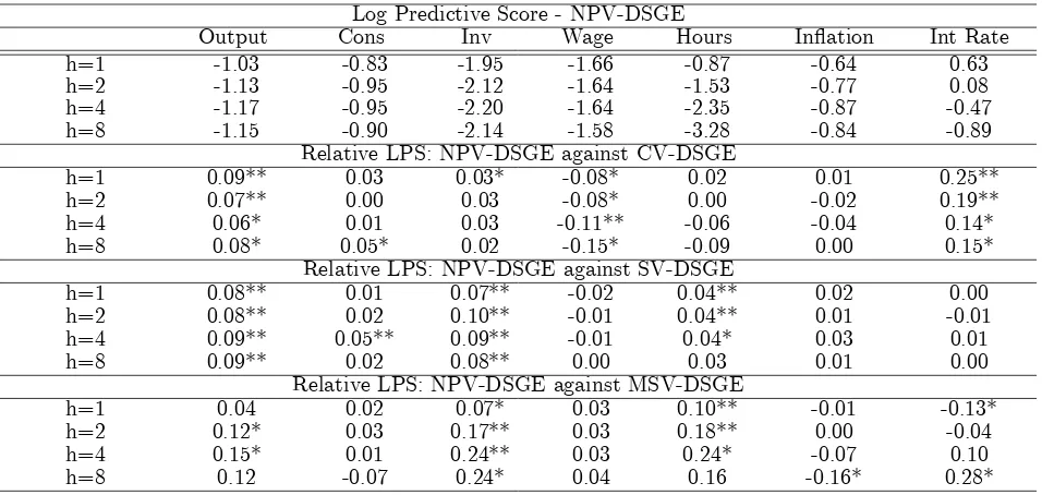
di¤erent from each other at 95%. Table 1 evaluates the quality of the density forecasts measured

by log predictive score (LPS). The table displays absolute LPS for the NPV-DSGE model and

di¤erences in LPS between the NPV-DSGE and the alternative CV-, SV- and MSV-DSGE models

respectively, so positive numbers imply superior performance of our NPV-DSGE approach.

Log Predictive Score - NPV-DSGE

Output Cons Inv Wage Hours In‡ation Int Rate

h=1 -1.03 -0.83 -1.95 -1.66 -0.87 -0.64 0.63

h=2 -1.13 -0.95 -2.12 -1.64 -1.53 -0.77 0.08

h=4 -1.17 -0.95 -2.20 -1.64 -2.35 -0.87 -0.47

h=8 -1.15 -0.90 -2.14 -1.58 -3.28 -0.84 -0.89

Relative LPS: NPV-DSGE against CV-DSGE

h=1 0.09** 0.03 0.03* -0.08* 0.02 0.01 0.25**

h=2 0.07** 0.00 0.03 -0.08* 0.00 -0.02 0.19**

h=4 0.06* 0.01 0.03 -0.11** -0.06 -0.04 0.14*

h=8 0.08* 0.05* 0.02 -0.15* -0.09 0.00 0.15*

Relative LPS: NPV-DSGE against SV-DSGE

h=1 0.08** 0.01 0.07** -0.02 0.04** 0.02 0.00

h=2 0.08** 0.02 0.10** -0.01 0.04** 0.01 -0.01

h=4 0.09** 0.05** 0.09** -0.01 0.04* 0.03 0.01

h=8 0.09** 0.02 0.08** 0.00 0.03 0.01 0.00

Relative LPS: NPV-DSGE against MSV-DSGE

h=1 0.04 0.02 0.07* 0.03 0.10** -0.01 -0.13*

h=2 0.12* 0.03 0.17** 0.03 0.18** 0.00 -0.04

h=4 0.15* 0.01 0.24** 0.03 0.24* -0.07 0.10

h=8 0.12 -0.07 0.24* 0.04 0.16 -0.16* 0.28*

Table 1. Log Predictive Score. The …gures in the top panel are the LPS of the NPV-DSGE model, the …gures under the remaining models are di¤erences between the LPS of the NPV-DSGE, and CV-, SV- and MSV-DSGE speci…cations respectively. ‘*’ and ‘**’ indicate rejection of the null of equal performance against a two-sided alternative at 5% and 1% signi…cance level respectively, using a Diebold-Mariano test.

With the exception of the wage growth, our NPV-DSGE model delivers statistically signi…cant

improvements for most variables and horizons over both CV-, SV- and MSV-DSGE speci…cations.

Outperforming the CV-DSGE model is expected, especially since the out-of-sample contains periods

performance between the SV-DSGE and NPV-DSGE models can be accounted for by recalling that

the NPV-DSGE model’s volatility estimates are much smoother, as illustrated in Figure 1, while

the SV-DSGE delivers more noisy and ragged estimates. In particular, the LPS performance of

the NPV-DSGE model is statistically superior at 1% signi…cance level than that implied by the

SV-DSGE model for output and investment growth for all horizons, which are key variables to

forecast. This is a consequence of the NPV-DSGE approach uncovering more time variation in

the TFP shock’s volatility which a¤ects consumption, investment and output forecasts through

the production function and the resource constraint of the Smets and Wouters (2007) model. The

superior performance of our NPV-DSGE model over the MSV-DSGE speci…cation is due to i) the

oversimpli…ed way in which volatility enters the MSV-DSGE model (i.e. two common volatility

states for all seven shocks), and ii) the Markov switching nature of the volatility process being

subject to abrupt changes rather than smooth time variation.

5

Conclusion

In this paper we propose a novel quasi-Bayesian Metropolis-within-Gibbs algorithm for the

estima-tion of changing volatility in DSGE models. The estimaestima-tion is based on previous work of Petrova

(2017) and di¤ers from existing approaches in being nonparametric and, as a consequence, valid

under possible misspeci…cation of the law of motion of the volatility, ensuring consistent estimation

in a wide class of deterministic and stochastic processes. The proposed approach delivers a

condi-tional quasi-posterior for the drifting volatilities of an inverse-Wishart form which gives rise to a

novel Metropolis-within-Gibbs algorithm. The availability of a closed form expression for the

quasi-posterior makes our algorithm computationally simpler than existing algorithms that are based on

a combination of Kalman …ltering and Kim et al. (1998)’s procedure.

We apply our estimation procedure to the Smets and Wouters (2007) model and show that the

estimated volatilities of the structural shocks exhibit slower time variation compared to

alterna-tive approaches. In addition, we demonstrate that the algorithm developed in this paper delivers

statistically signi…cant improvements to the density forecasts of the model in comparison to the

stochastic volatility and Markov switching approaches respectively.

References

Benati, L. and Surico, P. (2009). VAR analysis and the Great Moderation,American Economic Review99(4): 1636–1652.

Blanchard, O. J. and Kahn, C. M. (1980). The solution of linear di¤erence models under rational expectations,Econometica

48(5): 1305–1312.

Canova, F. and Gambetti, L. (2009). Structural changes in the US economy: Is there a role for monetary policy,Journal of Economic Dynamics and Control33(2): 477–490.

Carter, C. K. and Kohn, R. (1994). On Gibbs sampling for state space models,Biometrica81: 541–553.

Cogley, T. and Sargent, T. J. (2005). Drifts and volatilities: Monetary policies and outcomes in the post World War II US,

Review of Economic Dynamics8: 262–302.

Cogley, T. and Sbordone, A. M. (2008). Trend in‡ation, indexation, and in‡ation persistence in the new Keynesian Phillips curve,American Economic Review95(5): 2101–2126.

Diebold, F. X., Schorfheide, F. and Shin, M. (2017). Real-time forecast evaluation of dsge models with stochastic volatility,

Journal of EconometricsForthcoming.

Durbin, J. and Koopman, S. (2002). A simple and e¢ cient simulation smoother for state space time series analysis,Biometrika

89(3): 603–616.

Fernandez-Villaverde, J. and Rubio-Ramirez, J. F. (2013). Macroeconomics and volatility: Data, models, and estimation,in

D. Acemoglu, M. Arellano and E. Dekel (eds),Advances in Economics and Econometrics: Tenth World Congress, Vol. 3, Cambridge University Press, pp. 137–183.

Fernandez-Villaverde, J., Rubio-Ramirez, J. and Uribe, M. (2011). Risk matters: The real e¤ects of volatility shocks,American Economic Review101(6): 2530–61.

Gali, J. and Gambetti, L. (2009). On the sources of the Great Moderation,American Economic Journal1(1): 26–57.

Giraitis, L., Kapetanios, G., Wetherilt, A. and Zikes, F. (2016). Estimating the dynamics and persistence of …nancial networks, with an application to the Sterling money market,Journal of Applied Econometrics31(1): 58–84.

Giraitis, L., Kapetanios, G. and Yates, T. (2014). Inference on stochastic time-varying coe¢ cient models,Journal of Econo-metrics179(1): 46–65.

Hastings, W. (1970). Monte Carlo sampling methods using Markov chain and their applications,Biometrika57: 97–109.

Justiniano, A. and Primiceri, G. E. (2008). The time-varying volatility of macroeconomic ‡uctuations,American Economic Review98(3): 604–641.

Kim, S., Shephard, N. and Chib, S. (1998). Stochastic volatility: likelihood inference and comparison with ARCH models,

Review of Economic Studies65: 361–393.

Liu, Z., Waggoner, D. F. and Zha, T. (2011). Sources of Macroeconomic Fluctuations: A Regime-Switching DSGE Approach,

Quantitative Economics, Econometric Society2(2): 251–301.

Metropolis, N., Rosenbluth, A., Rosenbluth, M., Teller, A. and Teller, E. (1953). Equation of state calculations by fast computing machines,Journal of Chemical Physics21(6): 1087–1092.

Mumtaz, H. and Surico, P. (2009). Time-varying yield curve dynamics and monetary policy,Journal of Applied Econometrics

24(6): 895–913.

Petrova, K. (2017). A quasi-bayesian local likelihood approach to time varying parameter VAR models,Working Paper.

Primiceri, G. (2005). Time-varying structural vector autoregressions and monetary policy, Review of Economic Studies

72(3): 821–852.

Schorfheide, F. (2000). Loss function-based evaluation of DSGE model,Journal of Applied Econometrics15(6): 645–670.

Sims, C. (2002). Solving linear rational expectations models,Computational Economics20(1-2): 1–20.

Sims, C. A. and Zha, T. (2006). Were there regime switches in U.S. monetary policy?,American Economic Review96: 1193– 1224.