arXiv:1206.0126v1 [astro-ph.SR] 1 Jun 2012
DOI: 10.1007/•••••-•••-•••-••••-•
Study of the three-dimensional shape and dynamics
of coronal loops observed by
Hinode
/EIS.
Solar Physics
P. Syntelis1 ·C. Gontikakis1 ·
M.K. Georgoulis1 ·C.E. Alissandrakis2 · K. Tsinganos3,4
c
Springer••••
Abstract We study plasma flows along selected coronal loops in NOAA Ac-tive Region 10926, observed on 3 December 2006 with Hinode’s EUV Imaging Spectrograph (EIS). From the shape of the loops traced on intensity images and the Doppler shifts measured along their length we compute their three-dimensional (3D) shape and plasma flow velocity using a simple geometrical model. This calculation was performed for loops visible in the Fe viii 185 ˚A, Fe x184 ˚A, Fexii 195 ˚A, Fe xiii 202 ˚A, and Fe xv 284 ˚A spectral lines. In most cases the flow is unidirectional from one footpoint to the other but there are also cases of draining motions from the top of the loops to their footpoints. Our results indicate that the same loop may show different flow patterns when observed in different spectral lines, suggesting a dynamically complex rather than a monolithic structure. We have also carried out magnetic extrapolations in the linear force-free field approximation using SOHO/MDI magnetograms, aiming toward a first-order identification of extrapolated magnetic field lines corresponding to the reconstructed loops. In all cases, the best-fit extrapolated lines exhibit left-handed twist (α <0), in agreement with the dominant twist of the region.
Keywords: Active Regions, Structure, Velocity Field, Magnetic fields.
1
Research Center for Astronomy and Applied Mathematics, Academy of Athens,
Soranou Efesiou 4, 11527, Athens, Greece email:[email protected]
email:[email protected]
2
Section of Astro-Geophysics, Department of Physics, University of Ioannina, 45110 Ioannina, Greece email: [email protected]
3
National Observatory of Athens,
Lofos Nymphon, Thission 11810, Athens Greece
4
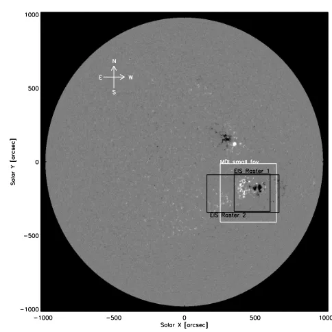
Figure 1. Full disk image recorded by SOHO/MDI on 3 December 2006, at 20:51 UT. EIS rasters 1 and 2 field of views are represented with dark frames around AR 10926. The white frame shows the part of the MDI magnetogram used for the magnetic field extrapolation.
1. Introduction
Solar telescopes provide us with two-dimensional projections of coronal struc-tures on the plane of the sky. The measure of the 3D geometry of coronal loops is important for understanding these structures. Reconstructions of a loop’s true shape have been attempted via a variety of methods, such as stereoscopy or
mod-els that make assumptions for the loop shape, flow etc (Loughhead, Wang, and Blows, 1983;
Berton and Sakurai, 1985; Aschwandenet al., 1999; Nitta, van Driel-Gesztelyi, and Harra-Murnion, 1999). Moreover, the STEREO space mission, with its twin telescopes in two different
positions in space, is dedicated to the solar coronal stereoscopy by combining simultaneous EUV images from two different lines of sight (Aschwanden, 2009; Aschwanden and W¨ulser, 2011). The 3D geometry of active-region loops, com-puted with STEREO images, was used to constrain the magnetic field topology computed with non-linear force-free extrapolation methods (De Rosaet al., 2009). To interpret the active-region Doppler maps computed with the data from in-struments such asHinode/EIS and to understand the plasma flows along coronal loops, one also needs to know the loops’ 3D geometry. Del Zanna (2008), using Hinode/EIS observations of NOAA AR 10926, studied the behavior of the line of sight velocity, along loops and weak emission regions of the active region, at different plasma temperatures.
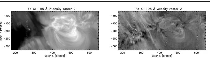
Figure 2. Left: EIS intensity image of the active region in Fexii 195 ˚A for raster 2. Right:
The corresponding EIS dopplergram. For the dopplergram, white/black colors corresponds to red/blue shifts. Doppler shifts are in the range of -20 to 20 km s−1
.
method, introduced by Alissandrakis, Gontikakis, and Dara, 2008 (Paper I) also uses the Doppler shifts measured along coronal loops in this reconstruction. Based on the analysis of Paper I we extend the study to more loops and a wider range of formation temperatures in this work.
2. Observations
NOAA AR 10926 was observed on 3 December 2006, at (395′′, -198′′) from disk center (see Figure 1). During that day,Hinode’s EUV Imaging Spectrograph (EIS) performed two rasters of the AR, recording spectral lines of Feviii 185 ˚A, (105.8K), Fex 184 ˚A, (106K), Fexii 195 ˚A, (106.1K), Fexiii 202 ˚A, (106.2K),
and Fexv 284 ˚A, (106.3K). These formation temperatures have been published by Young et al., 2007. Raster 1 was obtained from 15:32:19 UT to 17:46:31 UT with a 256′′ × 256′′ field of view (FOV), while raster 2 was obtained from 19:15:12 UT to 23:44:09 UT and covered a 512′′×256′′FOV Both rasters were scanned from West to East (see Figure 1) with a 30 s exposure time for each slit position, and a 1′′ spatial pixel size. We also used a timeseries of TRACE 171 ˚A filtergrams, recorded from 19:10:49 UT to 23:49:06 UT, with 0.5′′spatial pixel size and a time cadence of 1 minute. Magnetic field extrapolations were performed using a SOHO/MDI magnetogram. The MDI full disk line-of-sight magnetogram (Figure 1) has a rough pixel size of 1.9′′ but covered the entire active-region field-of-view and was recorded on 3 Dec. 2006 at 20:51:01 UT, during raster 2. SOT provided a vector magnetogram with a pixel size of 0.15′′ in a FOV of 316′′ ×157′′, pointing at (447′′,-171′′), that was taken on 4 Dec 2006, from 10:07:00 UT to 13:03:36 UT.
3. Data processing and loop reconstruction
fit was performed to estimate the effect of the blending on the dopplergrams. As the loops selected in Fe xii195 ˚A were outside the active region core, the Nixvi 185.23 ˚A line intensity is negligible, and does not influence the measured Doppler shift.
To calibrate the zero level of the measured Doppler shifts, we averaged the velocities in small quiet areas near the active region observed during the second raster. We compared our dopplergrams with the ones published in Del Zanna (2008) and found that they were in good agreement.
For every spectral line, pointing corrections relative to Heii 256 ˚A were taken into account to co-align the EIS data. Furthermore, in order for the different data sets to be comparable, co-alignment was performed among the EIS, TRACE, SOT and MDI data, within the uncertainty of the MDI spatial resolution.
From the aforementioned EIS data we manually selected, at each wavelength, the loops that could be distinguished from the background, along their entire length (Figure 3). For each loop, we recorded their positions (xs, ys) on the
intensity image as well as the Doppler shifts VSz, at the same positions, from
the Dopplergrams. We applied a boxcar average with a width of 5 to 7 at these line of sight velocities to reduce noise.
The measured positions (xs, ys) and line-of-sight velocities VSz along the
loops’ length, were then used as input for the computation of the loops’ 3D structure following the methodology of Paper I. Briefly, the model assumes that a given loop is (i) stationary, (ii) lying in a single plane, and (iii) exhibits plasma flows along its length. The sought-after unknown parameter is the inclinationβ of the plane with respect to the local solar vertical. There are two extremes for β: β1, that is the line-of-sight inclination with respect to the local vertical, and
a maximum inclinationβ2=β1−90◦such that the loop plane is not submerged
below the solar surface.
To find the unknown inclinationβ we first transform the loop’s positions and line-of-sight velocities from the sky coordinate system (xs, ys, zs) to the local
orthogonal system (xl, yl, zl), where the (xl, yl)-plane is tangent to the solar
surface andxlruns parallel to the equator, and then to the loop’s system (x, z).
Here ˆxis defined by the loop’s footpoints, ˆz is lying on the loop’s plane, and V(s, β) is the velocity on the plane, along the loop’s length (see Figure 3 of Paper I for the geometrical setup).
We apply the method by changing the inclination within the interval [β1, β2]
in steps of 0.1◦. At each step, we monitor the quantity
M(β) =max∆V(s, β), where ∆V(s, β) =|V(si+1, β)−V(si, β)|is the
abso-lute velocity difference between consecutive pixel positions, i, i+1, along the loop. The optimalβ is the one minimizingM(β). We further define an uncertaintyδβ such thatM(β) is smaller than, twice the minimumM(β)-value. In effect this is a 2−σuncertainty level; see Figure 4c for an example. Mostβ-values within the inspected range are immediately discarded either because large discontinuities appear inV(s, β) along the loop or becauseV(s, β) obtains unrealistically large values. Besides the primary minimumM(β) forβ ∈[β1, β2] we sometimes obtain
a secondary minimum forβ ≃β1. This is also typically discarded as the
Figure 3. Intensity images, in various spectral lines, from both rasters, on which we indicate the shape of the selected loops. Loop 1 appears in all lines and in all rasters. Loop 2 can be seen in panels a and e, Loop 3 in panels b and f, Loop 4 in panels c and g, loops 5 and 6 in panels d and h.
4. Results
In the studied active region, during both rasters and in all recorded spectral lines, we were able to identify six loops having a sufficient contrast with respect to the background along their entire length. All of them were located in the south part of the active region (solar-Y coordinates less than -200′′). For an additional four loops the method did not work successfully, failing to converge to a continuous velocity solution.
Figure 3 shows all studied loops as they appear in intensity images of different spectral lines during the two rasters. Loop 1 was the most prominent, as it appears in both rasters and in all wavelengths shown in Figure 3. Loop 2 was observed during raster 1 in Fexiii 202 ˚A and Fexii 195 ˚A (Figure 3 panels a,e). Loop 3 was observed during raster 2 in Fexv 284 ˚A and Fexiii 202 ˚A (Figure 3 panels b,f). Loop 4 was observed in Fex 184 ˚A during both rasters (Figure 3 panels c,g). Finally, loops 5 and 6 were observed in Feviii 185 ˚A during raster 1 and in Fexii 195 ˚A during raster 2 respectively (Figure 3 panels d,h).
4.1. Results for Loop 1
4.1.1. Loop reconstruction
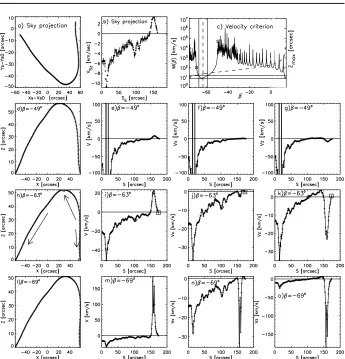
Figure 4. Results for Loop 1 at Fe xii 195 ˚A. First row, panels a and b: Loop position in
the sky plane and line-of-sight velocity as a function of the loop’s length. panel c, showsM(β) (solid line) and zmax(β), maximum loop altitude, (dashed line) as a function ofβ. The two
vertical lines show the range of optimum solutions while the vertical dashed line indicates the selectedβ. Each row of four panels shows calculations for different loop inclinations,β. These include: The reconstructed loop in its own plane (x, z) (panels d, h,l), the flow velocityV along the loop (panels e,i,m), the horizontal componentVx (panels f, j, n) and vertical component
Vz(panels g, k, o) as a function of the loop length. The third row is for the optimal value of
β=−63◦. The diamond indicates the top of the loop and the box indicates the west footpoint.
The arrows in panel h) show the direction of the plasma flow. Note the discontinuities of the flow velocity in the second and the fourth rows (β =−49◦and β =−69◦). Positive line of
sight velocities correspond to redshifts.
computed the loop shape and the velocity along the loop, in the loop reference system (x, z). Panel c) shows the maximum velocity difference (solid line)M(β) and the maximum loop altitude zmax (dashed line) as a function of β. Panel
(c) presents a ‘forest’ of large M(β) values, of the order of 103 to 106 km s−1
M(β) has another small value region, which corresponds to unphysically large values for zmax(≃10 000′′).
Each of the next three rows, has four panels, showing, from left to right, the reconstructed loop on its own plane, the velocityV of the flow along the loop, the horizontalVx and the verticalVz velocity components as a function of the
loop length. The second and fourth row show the results forβ=−49◦and−69◦ respectively. There, the transformation from the sky plane to the loop plane gives a discontinuity in the computed velocity (panels e, f and g) forβ=−49◦, and a strong peak in velocities that does not seem physical (panels m, n and o for β =−69◦), thus these results are rejected as unphysical. For the third row, where
β =−63◦, the velocity is continuous (panels i, j and k), and therefore the results are considered acceptable. The examined values of β range from β2 = −75◦
where the loop plane becomes tangent to the solar surface, to β1 = 14◦, where
the line-of-sight is inside the loop plane. Negative values of β means that the loop is inclined towards the south part of the active region. Let us come back to panel c. At β =−49◦ a square shows the M(β) value of 4.8×10⁴ km s−1
which corresponds to the subtraction between the most negative values ofvseen in panels (e), (f) and (g) at s= 19 arcsec, where V, Vx andVz resemble with
delta functions. Panel c), atβ=−69◦a square shows the value of≃105 km s−1
which corresponds to the maximum difference values ats≃155 arcsec in panels (m), (n) and (o).
The two horizontal lines show the minimum and two times the minimum of M(β). These yield a range for β (shown between the two continuous vertical lines), defining an uncertainty of ±4◦ for the loop’s inclination β. The mean value ofβ in this interval is pointed by the vertical dashed line.
4.1.2. Interpretation of flows in Loop 1
The flow velocityV, in Figure 4h, forβ=−63◦, is negative, with the exception of the west footpoint of the plot. This means that the velocity flow is towards the east footpoint starting from the upper part of the west leg, through the loop apex as indicated by the two arrows in panel h. There is however also a portion of the loop, near the west footpoint where we observe a downflow indicated by the right arrow in panel h. In panelj, Vx, is negative, indicating also a motion
towards the east footpoint. The west leg is almost vertical which is whyVx≃0.
In panel k,Vz also shows a flow towards the east footpoint with
negative/down-flows, east of the loop top (diamond), and positive/up-flows west of the loop top. Near the west footpoint,Vz changes sign again, at the same position where also
the Doppler shift changes sign (panel b). This would mean that the plasma flows towards the west footpoint in this small section. However, the small Doppler shift values increase the relative error and makes interpretation ambiguous, for this small loop section.
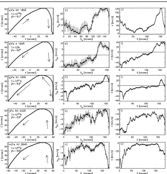
Figure 5. Results for Loop 1 for all spectral lines during Raster 2. First column: The recon-structed loop in its own plane (x, z). Second column: Line-of-sight velocity as a function of the loop’s length. Third column: Velocity of the flow as a function of the reconstructed loop’s length.
From the first column of panels we can see that Loop 1 implies similar inclina-tions in all spectral lines, in the range of−63◦to−60◦. For the Feviii spectral line, we measure redshifts of 5 to 20 km s−1 along the loop (panel b) which for
the given loop inclination correspond to unidirectional flow from the east toward the west footpoint (panel c). The results for Fe x spectral line, show that both the Doppler shift (panel e) and the computed velocity (panel f) change sign near the loop top; this indicates a draining motion from the loop top (indicated with a diamond symbol) towards the footpoints. This draining shows velocities of ≃40 km s−1 at both footpoints. The last two spectral lines, Fexiii 202 ˚A and
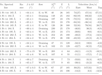
Table 1. A summary of the 3D reconstruction results for all selected loops. The Table includes: loop number (column 1), spectral line (column 2), raster number (column 3),β (column 4), the type of flow, which can be draining, or flow from East to West (E. to W.) or West to East (column 5), apparent density scale length (column 6) maximum altitude (column 7) and length (column 8). The last three columns, show the velocity mean values along 10% of the loops length starting respectively from east and the west footpoint and the mean velocity along 10% of the loop top. The corresponding standard deviation is shown in parenthesis.
No. Spectral Ra- β±δβ flow λobs
n Z L Velocities (km/s)
line ster (◦) (′′) (′′) (′′) East West Top
1 Feviii 185 ˚A 1 −64±4 E. to W. 40 26 185 74(27) 47(14) 47(11)
1 Fex 184 ˚A 1 −65±1 Draining 148 25 182 -92(19) 69(22) -1(3)
1 Fexii 195 ˚A 1 −65±1 Draining 197 23 176 -72(15) 33(12) -2(2)
1 Fexiii 202 ˚A 1 −65±1 W. to E. 221 23 176 -94(18) -36(14) -3(2)
1 Feviii 185 ˚A 2 −61±4 E. to W. 126 26 168 52(16) 76(34) 26(7)
1 Fex 184 ˚A 2 −60±4 Draining 230 25 170 -46(6) 36(3) -8(3)
1 Fexii 195 ˚A 2 −63±4 W. to E. 253 24 174 -30(6) 9(6) -6(1)
1 Fexiii 202 ˚A 2 −63±4 W. to E. 252 25 180 -40(2) -17(4) -12(1)
1 Fexv 284 ˚A 2 −64±2 W. to E. 272 26 190 -43(10) -21(3) -6(.5)
2 Fexii 195 ˚A 1 −64±4 Draining 47 15 129 -34(4) 19(6) -4(2)
2 Fexiii 202 ˚A 1 −64±4 W. to E. 102 15 129 -42(7) -9(12) -7(2)
3 Fexiii 202 ˚A 2 −75±15 W. to E. 205 4 64 -16(1) -11(3) -16(1)
3 Fexv 284 ˚A 2 −61±6 W. to E. 107 6 55 -11(1) -17(5) -7 (1)
4 Fex 184 ˚A 1 −69±7 Draining 66 7 73 -33(6) 31(4) -9(5)
4 Fex 184 ˚A 2 −65±7 W. to E. 177 9 65 -39(4) -21(2) -6(2)
5 Feviii 185 ˚A 1 −67±0.3 E. to W. 67 27 185 30(25) 147(32) 31(5)
6 Fexii 195 ˚A 2 −68±5 W. to E. 56 24 106 -14(2) 3(4) -12(2)
Fe xii 195 ˚A in panel (i), has also the characteristics of a unidirectional flow as in panels (l) and (o) but the positive flow at the west footpoint makes this interpretation problematic. It is worth noting that the flow in the hot lines is in the opposite direction to the flow in the cooler Feviii185 ˚A. Therefore, this may imply that Loop 1 is composed of different strands or background structures.
4.2. Results for all loops
loop 3 (line 12) and is of±15◦. In column 5 more than half of the loop (53%) show unidirectional flow from West to East, 30% show draining flow from the loop top to the footpoints while the rest of them, all in Feviii 185 ˚A line, have flows from East to West. Three of the four cases observed in the Fex 184 ˚A line presented draining motions.
We note that the dynamics of Loop 1 does not change qualitatively from the first to the second raster, except for the case of the Fe xii 195 ˚A line. Loops 4, 5 and 6 also change dynamics from the first to the second raster. For the cases with qualitatively similar loop dynamics in both rasters we can argue for a quasi-steady flow along them between 16:05 UT, the time when the first raster started scanning the loop, and 21:31 UT, the time the second raster finished, which is five and a half hours. Moreover, the ratios of the loop lengths (Table 1, column 8) over the corresponding velocities at the footpoints (columns 9 and 10), give timescales, 90% of which, are within 25 minutes to 2 hours. These values are close to the duration of the loops rastering (about 1 hour). For the other loops we cannot argue whether or not their dynamical behavior changes between the two rasters. However, as long as the loop magnetic structure is not modified during the raster, the applied method should give valuable results for the inclinationβ.
The last three columns of Table 1 show the velocity average values along 10% of the loop’s length starting, respectively, from the east footpoint the west footpoint and at the top of the loop, with their standard deviation in parenthesis. In most cases, the east footpoints have larger velocities by, factors from 1.2 to 3. We suggest that the loops appearing in Fe xiii 202 ˚A and Fe xv 284 ˚A should correspond to the same loop because the calculated dynamics is very similar. Columns 7 and 8 show the maximum altitude from the solar surface and the true loop lengths respectively. Loop 1 is apparently composed of separate strands that appear in different spectral lines as indicated by the different kind of flows found. For each spectral line, the reconstructing method gave values of the loop height (column 7) which vary from 23′′to 26′′while the loop reconstructed length varies from 170′′to 190′′. These variations indicate the uncertainties of the method but could also show the difference between various strands composing the loop.
4.2.1. Calculation of length scales and Mach numbers
The hydrostatic pressure scale height, defined in centimeters as (λp = 4.7×
109(T /1M K)), (Aschwanden, 2005) for the spectral lines Feviii, 185 ˚A, (105.8K), Fe x, 184 ˚A, (106 K), Fexii, 195 ˚A, (106.1 K), Fe xiii, 202 ˚A, (106.2 K), and Fe xv, 284 ˚A (106.3 K), is 41.5′′, 65.7′′, 82.7′′, 104.2′′, and 131.2′′respectively, and was computed using the formation temperature of each spectral line given in the parentheses. This scale height is still meaningful for subsonic flows which is the case of our loops as it is shown in the next paragraph. Note that the maximum altitudes (column 7) of all measured loops are smaller than the corresponding pressure scale height. Thus this explains that the tops of loops are dense enough to be bright and detectable.
Column 6 shows the apparent density scale, λobs
n (see Aschwanden, 2005 p.
84). To calculateλobs
the background contamination. To estimate the background, we represented each loop in images with curvilinear grids, (Aschwandenet al., 1999 their Figure 6). The x-axis of these images represents the length along the loop so that the loop looks stretched and horizontal. For each point (xloop, yloop) along the loop
in the curvilinear grid, we selected pixels lying along the line perpendicular to the loop (xloop, y) with intensities Iback(xloop, yback) < f Iloop(xloop, yloop)
where factor f is in the range from 0.5 to 0.8. We subtract the average of the background pixels intensities from the corresponding loop pixel intensities to get the corrected intensity along the loop. We then calculate the electron density ne(s) along the loop as follows. For each loop we use the contribution
functions G(T) of the corresponding spectral line from the CHIANTI software (Dere et al., 1997). The contribution function for all spectral lines was computed assuming a Mazzottaet al., 1998 ionization fraction and a hybrid abundance for iron (Fludra and Schmelz, 1999). We assume that the loop width along the line of sight is constant and of w = 2′′. The electron density is calculated as
ne(s) =
q I(s)
wG(Tmax).Tmaxis the spectral lines formation temperature,
maximiz-ing the contribution function andsis the length along the loop. We performed a fit with an exponential function to the electron density functionne(s) computed
along the loop. The density scale length λobs
n is the derived length from the
exponential fit. The resulting relative difference betweenλobs
n andλp/cos(β) is
in the range of 0.01 to 0.8 with an average of 0.46. The sound velocity, expressed as vs = 0.151×
√
T km s−1, was computed
for the different spectral lines formation temperatures to be in the range of 120 km s−1 to 213 km s−1. Therefore, the corresponding Mach numbers, are
smaller than one with the exception of the west footpoint of loop 5 (row 15 in Table 1) which is supersonic. For the Fe viii, 185 ˚A, Fe x, 184 ˚A, Fe xii, 195 ˚A, Fe xiii, 202 ˚A and the Fe xv, 284 ˚A lines, the mean Mach numbers computed from the corresponding velocities in columns 9 and 10 (Table 1) are 0.6, 0.3, 0.2, 0.2 and 0.1 respectively and shows that, the larger the line formation temperature the smaller the Mach number.
4.2.2. Influence of background correction on Doppler shifts
In order to check the influence of the background on our results, we also per-formed the loop reconstruction, using loop Doppler shifts calculated from
spec-tral profiles from which we subtracted a background specspec-tral profile (Gontikakiset al., 2005). We got better results when the background points were selected along the same
5. Comparing reconstructed with extrapolated coronal-loop shapes
As an independent test of our 3D reconstructions we used linear force-free magnetic field extrapolations as described by Alissandrakis (1981) to deter-mine whether extrapolated field lines (viewed as loops) that model the recon-structed loops can be found. That active-region magnetic fields are far from a linear force-free configuration (and, in fact, far from a force-free field config-uration in general, at least at photospheric heights) is well known (see, e.g., Metcalfet al., 1995; Georgoulis and LaBonte, 2004). However, we are seeking singleα-values to fitsingleloops, with different values corresponding to different loops. In this approach we have better control over the fitting process, that cannot be achieved by a fully-fledged model-dependent nonlinear force-free field extrapolation (see, e.g., Schrijveret al., 2006; Metcalfet al., 2008). To compare the observed and the extrapolated loops we employ the distance modulus Cl,
introduced by (Wiegelmann and Neukirch, 2002), namely,
Cl=
1 L2
loop Z
|Rloop−Rline|dl , (1)
where Rloop,Rline are respective vector positions along the reconstructed loop and extrapolated field line, respectively, and Lloop is the loop’s length.
In-tegration occurs along the reconstructed loop’s length with respective points considered as points having the same location (in terms of normalized distance from footpoints) along the loop. The number of points taken vary with the loops’ length: for the smallest loop (loop 3) we used 51 points while for the largest (loops 1 and 5) we used up to 215 points. We only compared loops and extrapolated field lines with footpoints lying within a square with a 30′′-linear size.
As lower boundaries for the extrapolations we use a Level 1.8 magnetogram from the full-disk Michelson Doppler Imager (MDI; Scherreret al., 1995) on-board SOHO. The course of action is to, first, crop the MDI magnetogram to select the desired photospheric patch and then use the cosine-corrected line-of-sight magnetic field component on the image (sky) plane. We choose this action because de-projecting for the local, heliographic plane would introduce unfore-seen uncertainties when similarly de-projecting the EIS images. Point taken, we understand that each approach has weaknesses – this is an issue that we plan to investigate thoroughly in future studies.
The linear size of the selected patch isL= 183 Mm. This determines the ex-tremes of the|α|-range to be investigated (e.g., Alissandrakis, 1981; Greenet al., 2002), by the formula |αmax| = (2π/L). Hence, we scan an α-range between
−0.0343M m−1 and 0.0343M m−1, with a step-size equal to 0.006M m−1.
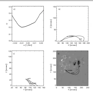
An example loop fitting, corresponding to Loop 1 at Fe xii 195 ˚A is shown in Figure 6. The minimumCl-value achieved in this case (Figure 6a; also shown
in Table 2) isCl≃0.2. Figure 6 also includes the best-fit extrapolated field line
Figure 6. Fitting Loop 1 at Fexii 195 ˚A during raster 1: (a) theClmodulus along the loop
as a function ofα. A minimumClis achieved forα≃ −0.009M m−1. (b, c) Two different
views of the inferred loop (thick solid curve), accompanied by a potential-field extrapolated line (α= 0; dotted curve) and the ”best-fit” extrapolated field line (α=−0.009M m−1
; thin solid curve). (d) The same system, seen from above and projected on the respective SOHO/MDI magnetogram.
to the distances between the two (loop and field-line) apices. In addition, the Cl-curve is quite shallow (as also reported by Wiegelmann and Neukirch, 2002)
so different α-values give rise to very similar extrapolated lines. In situations like this it is challenging to assign an uncertainty to each best-fit value. For the purpose of providing an error margin in the best-fitα-values, however, we have selected a 10%-margin inClenclosing the minimum and calculated the standard
deviations ofα-values within this margin. For the example of Figure 6 we find α = −0.009±0.006 Mm−1. Even given the uncertainty, therefore, Loop 1 at
Fexii 195 ˚A is better fitted by a negative-αfield line.
From the 17 loop cases listed in Table 1 the fitting method gave a minimum (albeit shallow) Cl in 15 cases. The results are summarized in Table 2. From
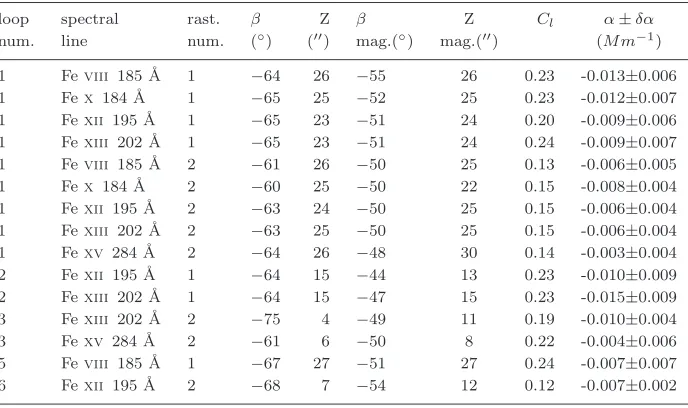
well-Table 2. Summary of the results obtained from the magnetic field extrapolation in comparison to the results of the 3D reconstruction. Columns 4 and 5 are the reconstruction results as in Table 1. Columns 6 to 8 are the extrapolation results for the best fitting magnetic line and column 9 is the calculated bestαwith its error bar.
loop spectral rast. β Z β Z Cl α±δα
num. line num. (◦) (′′) mag.(◦) mag.(′′) (M m−1
)
1 Feviii 185 ˚A 1 −64 26 −55 26 0.23 -0.013±0.006
1 Fex 184 ˚A 1 −65 25 −52 25 0.23 -0.012±0.007
1 Fexii 195 ˚A 1 −65 23 −51 24 0.20 -0.009±0.006
1 Fexiii 202 ˚A 1 −65 23 −51 24 0.24 -0.009±0.007
1 Feviii 185 ˚A 2 −61 26 −50 25 0.13 -0.006±0.005
1 Fex 184 ˚A 2 −60 25 −50 22 0.15 -0.008±0.004
1 Fexii 195 ˚A 2 −63 24 −50 25 0.15 -0.006±0.004
1 Fexiii 202 ˚A 2 −63 25 −50 25 0.15 -0.006±0.004
1 Fexv 284 ˚A 2 −64 26 −48 30 0.14 -0.003±0.004
2 Fexii 195 ˚A 1 −64 15 −44 13 0.23 -0.010±0.009
2 Fexiii 202 ˚A 1 −64 15 −47 15 0.23 -0.015±0.009
3 Fexiii 202 ˚A 2 −75 4 −49 11 0.19 -0.010±0.004
3 Fexv 284 ˚A 2 −61 6 −50 8 0.22 -0.004±0.006
5 Feviii 185 ˚A 1 −67 27 −51 27 0.24 -0.007±0.007
6 Fexii 195 ˚A 2 −68 7 −54 12 0.12 -0.007±0.002
reproduced by the fitting. Excluding Loop 3 at Fexiii 202 ˚A (7′′ of difference) and Loop 6 at Fe xii 195 ˚A (5′′ of difference), the mean amplitude difference inZ between loops and extrapolated field lines is (1.2±1.3)′′, corresponding to ∼5.5% of the mean loop length. When it comes to loop inclinations, however, extrapolation gives consistentlylower inclinations. The mean inclination differ-ence between all reconstructed loops and extrapolated field lines in Table 2 is 14.5◦±4.3◦, or (22.5±5)% of the reconstructed loop length. The reason(s) for this systematic difference need to be investigated further. Generally speaking, however, more than one effect may be contributing to this: besides the limited validity of the force-free approximation in the photospheric magnetic fields used as extrapolation boundaries that, however, is not clear whether should yield a systematic lower inclination, (i) the central assumption of loops lying in a single plane may overestimate the loops’ inclination as the most highly projected parts of each loop weigh heavier in the reconstruction, and (ii) the extrapolations using the image-plane magnetic field include some projections that may well give rise to an underestimation of the extrapolated field lines’ inclination.
[image:14.595.126.470.139.343.2]for the entire NOAA AR 10926 (α=−0.049±0.006M m−1), as calculated by
the method described in Georgoulis and LaBonte, 2007, using the SOT mag-netogram. This implies that the linear force-free method applied separately to each loop consistently yields a dominant left-hand twist in the AR, in agree-ment with the cruder linear force-free approximation for the entire AR. Even the systematic lower inclination for extrapolated field lines is an effect that is interesting to investigate further, as one may be able to assess the validity of the loop reconstruction methodvis ´a visvarious effects in the extrapolation. We intend to continue and extend these comparisons to clarify these issues.
6. Summary and Conclusions
We reconstructed the 3D geometry of six loops observed by the Hinode/EIS spectrograph in five spectral lines during two rasters of the instrument, a total of 17 cases. All loops correspond to NOAA AR 10926. All reconstructed loops have large inclinations with respect to the vertical, in the range of−60◦to−75◦ and they are all projected to the South of the bright central part of the active region. Moreover, due to pressure scale height effects, large inclinations lead to denser and brighter plasma near the loop top, hence the entire loop stands clearly above the background level. The flows calculated for all loops were subsonic in all spectral lines that validates the loops description using their hydrostatic scale.
The best-studied loop is Loop 1, successfully reconstructed in nine images. We find that this loop is not a monolithic structure, as the flows deduced in different spectral lines vary from unidirectonal flow from East to West in the low-temperature Feviii line, to draining motion from the top to the footpoints in the intermediate-temperature Fe x line, to unidirectional flow from West to East in the high-temperature lines. This being said, the computed inclination is very similar in all images, namely 63◦±3◦, that strengthens our assessment of internal structure in the loop in different temperature ranges.
An independent comparison between the reconstructed loops and extrapo-lated field lines by means of a linear force-free extrapolation implemented on a case-by-case basis give results that call for additional investigation. We have been able to closely model the height of the loops’ apices and we have noticed best-fit lines with a consistent (left-handed in this case) twist in the AR, but extrapolated field lines are consistently less inclined than reconstructed loops. This discrepancy may be due to drawbacks in the reconstruction method, weak-nesses in the extrapolation and/or the extrapolated boundary, or a combination of both. Aiming to validate our technique as reliably as possible, we intend to carry out similar investigations in future works, relying on larger statistical samples of reconstructed coronal loops.
References
Alissandrakis, C.E.: 1981, On the computation of constant alpha force-free magnetic field.
Astron. Astrophys.100, 197 – 200.
Alissandrakis, C.E., Gontikakis, C., Dara, H.C.: 2008, paper I: Determination of the True Shape of Coronal Loops.Solar Phys.252, 73 – 87. doi:10.1007/s11207-008-9242-4. Aschwanden, M.J.: 2005, Physics of the Solar Corona. An Introduction with Problems and
Solutions (2nd edition) Springer-Praxis Books / Astronomy and Planetary Sciences,
Chichester, UK; Springer, New York, Berlin.
Aschwanden, M.J.: 2009, The 3D Geometry, Motion, and Hydrodynamic Aspects of Oscillating Coronal Loops. Space Sci. Rev.149, 31 – 64. doi:10.1007/s11214-009-9505-x.
Aschwanden, M.J., W¨ulser, J.-P.: 2011, 3-D reconstruction of active regions with STEREO.J.
Atmosph. Solar-Terr. Phys.73, 1082 – 1095. doi:10.1016/j.jastp.2010.09.008.
Aschwanden, M.J., Newmark, J.S., Delaboudini`ere, J.-P., Neupert, W.M., Klimchuk, J.A., Gary, G.A., Portier-Fozzani, F., Zucker, A.: 1999, Three-dimensional Stereoscopic Analysis of Solar Active Region Loops. I. SOHO/EIT Observations at Temperatures of (1.0-1.5) ×106
K. Astrophys. J.515, 842 – 867. doi:10.1086/307036.
Berton, R., Sakurai, T.: 1985, Stereoscopic determination of the three-dimensional geometry of coronal magnetic loops.Solar Phys.96, 93 – 111. doi:10.1007/BF00239795.
Carcedo, L., Brown, D.S., Hood, A.W., Neukirch, T., Wiegelmann, T.: 2003, A Quantitative Method to Optimise Magnetic Field Line Fitting of Observed Coronal Loops.Solar Phys.
218, 29 – 40. doi:10.1023/B:SOLA.0000013045.65499.da.
De Rosa, M.L., Schrijver, C.J., Barnes, G., Leka, K.D., Lites, B.W., Aschwanden, M.J., Amari, T., Canou, A., McTiernan, J.M., R´egnier, S., Thalmann, J.K., Valori, G., Wheatland, M.S., Wiegelmann, T., Cheung, M.C.M., Conlon, P.A., Fuhrmann, M., Inhester, B., Tadesse, T.: 2009, A Critical Assessment of Nonlinear Force-Free Field Modeling of the Solar Corona for Active Region 10953. Astrophys. J.696, 1780 – 1791. doi:10.1088/0004-637X/696/2/1780. Del Zanna, G.: 2008, Flows in active region loops observed by Hinode EIS. Astron. Astrophys.
481, L49 – L52. doi:10.1051/0004-6361:20079087.
D´emoulin, P., Mandrini, C.H., van Driel-Gesztelyi, L., Thompson, B.J., Plunkett, S., K˝ov´ari, Z., Aulanier, G., Young, A.: 2002, What is the source of the magnetic helicity shed by CMEs? The long-term helicity budget of AR 7978. Astron. Astrophys.382, 650 – 665. doi:10.1051/0004-6361:20011634.
Dere, K.P., Landi, E., Mason, H.E., Monsignori Fossi, B.C., Young, P.R.: 1997, CHIANTI - An Atomic Database For Emission Lines - Paper I: Wavelengths greater than 50 ˚A. Astron.
Astrophys. Suppl.125, 149 – 173.
Fludra, A., Schmelz, J.T.: 1999, The absolute coronal abundances of sulfur, calcium, and iron from Yohkoh-BCS flare spectra. Astron. Astrophys.348, 286 – 294.
Georgoulis, M.K., LaBonte, B.J.: 2004, Vertical Lorentz Force and Cross-Field Currents in the Photospheric Magnetic Fields of Solar Active Regions. Astrophys. J. 615, 1029 – 1041. doi:http://dx.doi.org/10.1086/424501.
Georgoulis, M.K., LaBonte, B.J.: 2007, Magnetic Energy and Helicity Budgets in the Active Region Solar Corona. I. Linear Force-Free Approximation. Astrophys. J.671, 1034 – 1050. doi:10.1086/521417.
Gontikakis, C., Petie, G.J.D., Dara, H.C., Tsinganos, K.: 2005, A solar active re-gion loop compared with a 2D MHD model. Astron. Astrophys. 434, 1155 – 1163. doi:10.1051/0004-6361:20041268.
Green, L.M., L´opez Fuentes, M.C., Mandrini, C.H., D´emoulin, P., van Driel-Gesztelyi, L., Culhane, J.L.: 2002, The Magnetic Helicity Budget of a cme-Prolific Active Region.Solar
Phys.208, 43 – 68.
Loughhead, R.E., Wang, J.-L., Blows, G.: 1983, High-resolution photography of the solar chromosphere. XVII Geometry of H-alpha flare loops observed on the disk. Astrophys. J.
274, 883 – 899. doi:10.1086/161501.
Mazzotta, P., Mazzitelli, G., Colafrancesco, S., Vittorio, N.: 1998, Ionization balance for opti-cally thin plasmas: Rate coefficients for all atoms and ions of the elements H to NI. Astron.
Astrophys. Suppl.133, 403 – 409.
Metcalf, T.R., Jiao, L., McClymont, A.N., Canfield, R.C., Uitenbroek, H.: 1995, Is the solar chromospheric magnetic field force-free? Astrophys. J. 439, 474 – 481. doi:http://dx.doi.org/10.1086/175188.
Modeling of Coronal Magnetic Fields. II. Modeling a Filament Arcade and Sim-ulated Chromospheric and Photospheric Vector Fields. Solar Phys. 247, 269 – 299. doi:10.1007/s11207-007-9110-7.
Nitta, N., van Driel-Gesztelyi, L., Harra-Murnion, L.K.: 1999, Flare loop geometry.Solar Phys.
189, 181 – 198.
Scherrer, P.H., Bogart, R.S., Bush, R.I., Hoeksema, J.T., Kosovichev, A.G., Schou, J., Rosen-berg, W., Springer, L., Tarbell, T.D., Title, A., Wolfson, C.J., Zayer, I., and the MDI Engineering team: 1995, The Solar Oscillations Investigation - Michelson Doppler Imager.
Solar Phys.162, 129 – 188. doi:10.1007/BF00733429.
Schrijver, C.J., De Rosa, M.L., Metcalf, T.R., Liu, Y., McTiernan, J., R´egnier, S., Valori, G., Wheatland, M.S., Wiegelmann, T.: 2006, Nonlinear Force-Free Modeling of Coronal Magnetic Fields Part I: A Quantitative Comparison of Methods.Solar Phys.235, 161 – 190. doi:10.1007/s11207-006-0068-7.
Wiegelmann, T., Neukirch, T.: 2002, Including stereoscopic information in the reconstruction of coronal magnetic fields.Solar Phys.208, 233 – 251.