THE DETERMINATION OF ACTIVATION ENERGY
FROM LINEAR HEATING RATE EXPERIMENTS:
A COMPARISON OF THE ACCURACY OF ISOCONVERSION METHODS
M.J. Starink
Materials Research Group, School of Engineering Sciences, University of Southampton, Southampton S017 1BJ, UK
************************************************************************ This document is nearly identical to the paper published in 2003 as:
M.J. Starink, “The determination of activation energy from linear heating rate experiments: a comparison of the accuracy of isoconversion methods”, Thermochim. Acta, 2003, Vol. 404, pp. 163-176
Changes in this version are:
• few isolated typographical errors have been corrected • references have been updated
• figures are in colour
************************************************************************
Abstract
Model-free isoconversion methods are the most reliable methods for the calculation of activation energies of thermally activated reactions. A large number of these isoconversion methods have been proposed in the literature. A classification of these methods is proposed. Type A methods such as Friedman methods make no mathematical approximations, and Type B methods, such as the generalised Kissinger equation, apply a range of approximations for the temperature integral. The accuracy of these methods is investigated, by deriving expressions for the main sources of error which includes the inaccuracy in reaction rate measurement, approximations for the temperature integral and inaccuracies in determination of temperature for equivalent fraction transformed. Both highly inaccurate and highly accurate Type B methods are identified. In cases where some uncertainty over baselines of the thermal analysis data exists or where accuracy of determination of transformation rates is limited, type B methods will often be more accurate than type A methods.
1. Introduction
A general objective of the modelling of thermally activated reactions is the derivation of a complete description of the progress of a reaction that is valid for any thermal treatment, be it isothermal, by linear heating or any other non-isothermal treatment [1,2]. For many reactions this objective is a daunting one as any given reaction might progress through a range of mechanisms and intermediate stages, all of which can have a different temperature-dependency, and this is especially so for solid-state reactions. To come to terms with this potentially very complicated problem, most researchers attempt to achieve the objective by making a few judiciously chosen simplifying assumptions. A simplifying assumption that is encountered in innumerable publications is the assumption that the transformation rate during a reaction is the product of two functions, one depending solely on the temperature, T, and the other depending solely on the fraction transformed, α [3]:
) ( ) ( k T f
dt
dα= α (1)
The temperature dependent function is generally assumed to follow an Arrhenius type dependency.
⎟ ⎠ ⎞ ⎜
⎝ ⎛− =
RT E k
k oexp (2)
Thus, to describe the progress of the reaction at all temperatures and for all temperature-time programmes, the function f(α), and the constants ko and E need to be determined. In general, the reaction function f(α) is unknown at the outset of the analysis. A range of standard functions which represent particular idealised reaction models have been proposed (see e.g. [4,5]).
From Eqs. (1) and (2) follows immediately that for transformation studies by performing experiments at constant temperature, Ti, E can be obtained from the well-known relation:
1
ln C
RT E t
i
f= + (3)
where tf is the time needed to reach a certain fraction transformed, and C1 is a constant which depends on the reaction stage and on the kinetic model. Thus E can be obtained from two or more experiments at different T. For isothermal experiments k(T) is constant, the determination of f(α) is relatively straightforward, and is independent of E.
non-isothermal methods in general [22]. Some methods are non-transparent because they rely on numerical integration of data, which may explain the relatively scarce use of more recent less transparent methods. It is further noted that in many publications inaccuracies in some activation energy analysis methods introduced by approximation of the so-called temperature integral (see section 2.2) are cited as justification for the development of further new (and often non-transparent) models, without considering whether the magnitude of these inaccuracies are significant and mostly without providing proof that new methods are any more accurate than existing methods. In an attempt to clarify the current state of activation energy analysis, the present paper has two aims. First aim is to clarify the reasons behind the profusion of activation energy methods through analysing and categorising the derivations and approximations made. This will lead to a simple means of categorising isoconversion methods, which encompasses all known isoconversion methods. This work has also allowed identification of several new isoconversion methods, which have benefits over existing methods. The second aim is to provide a quantitative and conclusive analysis of the errors and uncertainties of a large number of isoconversion methods (including the best known ones), and thus unambiguously determine the benefits and drawbacks of the methods.
2 Methods for determination of activation energy.
For transformation studies performed at constant heating rate, a wide range of methods for deriving the activation energy of a reaction that conforms to Eqs. (1) and (2) have been proposed (a selection of methods can be found in [3-18]). All reliable methods of activation energy analysis require the determination of the temperatures, Tf(β), at which an equivalent stage of the reaction is obtained for various heating rates. Hence the term isoconversion methods. The equivalent stage (also called fixed or identical stage) may be defined as the stage at which a fixed amount is transformed, or at which a fixed fraction of the total amount is transformed [23]. Isoconversion methods can be categorised into one of two main groups of methods. One set of methods relies on approximating the so-called temperature integral and requires data on Tf(β) only. For reasons that will become clear below, will use the term p(y)-isoconversion methods to describe the methods in this category and class them as type B methods. This set of methods includes the Kissinger method [6,7], the Kissinger-Akahira-Sunose method [9] (also termed the generalised Kissinger method), the Flynn-Wall-Ozawa method [10,12,13] and 2 methods developed by the present author [15]. Another set of methods does not use any mathematical approximation, but instead uses a determination of the reaction rate at an equivalent stage of the reaction for various heating rates. Hence, we will term this group of methods rate-isoconversion methods, or type A methods. A well-known method of this type is the Friedman method.
2.1 Type A: Rate-isoconversion methods (or Friedman type methods)
[17], and in this work we will indicate them as type A methods. The method is derived by inserting Eq. (2) into Eq. (1) and taking the logarithm, yielding:
) ( ln dt
d
ln α f α
RT E
f
− −
= (4)
Thus if a range of linear heating experiments at different heating rates, β, are performed and the times at which a fixed stage of the reaction is achieved can be identified for each linear heating experiment, f(α) will be a constant. By measuring Tf and the transformation rate dα/dt at that fixed stage for each of the experiments, we can obtain E from the slope of plots of ln(dα/dt) versus 1/Tf. As dα/dt can be difficult to measure accurately, whilst the heating rate is much easier to determine accurately, one usually prefers to rewrite the latter equation to:
) ( ln dT
d
ln α β f α
RT E
f
− −
= ⎟ ⎠ ⎞ ⎜
⎝
⎛ (5)
Hence E is now determined from the slope of plots of ln(β dα/dt) versus 1/Tf. (The work by Gupta et al [18] further clarifies the derivation of the rate isoconversion method first derived by Friedman [17].) Thus the method does not require any assumption on f(α), i.e. it is a so-called model-free method.
Whilst this type A (rate-isoconversion) method avoids making mathematical approximations used in type B methods (see below), they introduce some new measurement uncertainties as the measurement of the rate of conversion, dα/dT, is sensitive to the determination of the baseline and calibration of the thermal analysis equipment.
2.2 Type B: p(y)-isoconversion methods
The procedures for deriving and applying p(y)-isoconversion methods can be illustrated well by considering the derivation of the Kissinger-Akahira-Sunose (KAS) method [6,7,9,10] (sometimes called the generalised Kissinger method), which is one of the best known p(y)-isoconversion methods. In this derivation, Eq. (2) is inserted in Eq. (1) and this is integrated by separation of variables:
∫
∫
∫
⎟⎟ = ∞ −⎠ ⎞ ⎜⎜
⎝ ⎛ − =
f f
y o T
o
dy y
y R
E k dT RT
E k
f d
2 0
0
) exp( exp
)
(α β β
α
α
(6)
where y = E/RT, yf = E/RTf , Tf is the temperature at an equivalent (fixed) state of transformation, and β is the heating rate. The integral on the right hand side is generally termed the temperature integral (some authors use ‘Arrhenius integral’ [24]), p(y):
) ( ) exp(
2 f
y
y p dy y
y
f
= −
∫
∞
Integrating in parts and truncating the series by assuming yf >>1 results in the following approximation for p(y) (see e.g. Ref. [10]):
2 ) exp( ) ( ) (
y y y
p y
p ≅ K = − (8)
The assumption yf >>1 is reasonable, since for the vast majority of solid-state reactions (and many other reactions) 15< yf <60. By taking the logarithm of Eq. (6) and using Eq. (8) one obtains:
f f o
y y R
E k f
d = + −
∫
20
1 ln ln
) ( ln
β α
α
α
(9)
At constant fraction transformed, α, this leads to:
2 2
ln C
RT E
Tf f
+ − =
β (10)
C2 and subsequent C3, C4, etc are parameters that are independent of T and β. According to the latter equation, plots of ln(Tf2/β) versus 1/Tf should result in straight lines, the slope of the straight lines equalling E/R. The method does not require any assumption on f(α), i.e. just like other type A and type B methods, it is a model-free method. This Kissinger-Akahira-Sunose (KAS) is essentially identical to the method described by Vyazovkin and co-workers [25,26]. (Note that this early method by Vyazovkin is different from a later model [27,28] derived by him. Note also that various authors [21,29] have in the past derived Eq. (10) using a specific reaction model, but, as shown above and elsewhere [4,10,15], this limiting assumption is not required.)
All p(y)-isoconversion methods involve the plotting of 1/Tf vs. a logarithmic function which depends on the heating rate and often the temperature. The latter logarithmic function depends on the approximation for the temperature integral used, which is different for the different p(y)-isoconversion methods. Thus, the approximation of the temperature integral is key to understanding the different methods and below these approximations will be considered.
The temperature integral and its approximations
A range of approximations of the temperature integral p(y) have been suggested in the literature, and here we will here consider the best known, the most cited and the most accurate approximations, as well as consider how these approximations relate to each other.
reactions that were mentioned but not analysed with thermal analysis are considered, the lower limit for y is 9. (This exceptionally low value of y occurs for nitriding and carburising of steel.) There are several reasons for the lack of reactions with y values outside this range. Firstly, reactions with a high activation energy will generally occur at high temperatures and vice-versa. This will tend to limit the occurrence of extremely low or extremely high values of y. Secondly, for diffusion controlled reactions the typical diffusion distance, ℓ, is given by ℓ = Dt , where D is the diffusion coefficient. D is generally given by:
⎟ ⎠ ⎞ ⎜ ⎝ ⎛− = RT E D D D
oexp (11)
and thus we find:
⎟⎟ ⎠ ⎞ ⎜⎜ ⎝ ⎛ − = = t D RT E y o D 2
ln l (12)
Again, extreme values of y are unlikely because: a) ℓ and t are limited due to practical considerations, and the lower limit for ℓ is defined by interatomic distance, b) larger diffusion distances, ℓ, will imply longer experiment times, t, c) the logarithmic function will limit variation. Thus there are sound physical reasons for expecting that there are upper and lower boundaries to the range of y values that can occur. The assessment shows that in searching for an approximation for p(y) only the range 9<y<100 is of practical significance, whilst the overwhelming majority of reactions occur for 15<y<60.
In considering the different mathematical expressions for the temperature integral we will first consider series expansions, which form the basis for less accurate approximations. Three important types of expansions are the asymptotic expansion after a single integration in parts:
( )
⎟⎟ ⎠ ⎞ ⎜⎜ ⎝ ⎛ − + − + − + − = ... ) ( ! 4 ) ( ! 3 ! 2 1 exp )( 2 2 3
y y y y y y
p (13)
Schlomilch’s expansion [30]
( )
(
)(
) (
)(
)(
)
⎟⎟ ⎠ ⎞ ⎜⎜ ⎝ ⎛ + + + − + + + + − + − = ... 4 3 2 4 3 2 2 2 1 1 ) 1 ( exp ) ( y y y y y y y y y yp (14)
and Lyon’s expansion [16]
( )
(
)
(
)
⎟⎟⎠ ⎞ ⎜⎜ ⎝ ⎛ + + + − + + + − = ( − ) ... 2 8 2 2 1 ) 2 ( exp ) ( 42 O y
y y y y y y y y
p (15)
( ) (
1 ( ) )( exp )
( g y
y y
y y
p +
+ − =
ω
)
(16)where ϖ is a constant (in Eqs. (13) to (15) equalling 0, 1 and 2), g(y) is a an expansion of which the first term is of the order y-1 or y-2, with g(y)<<1 (providing y is larger than about 10). It is apparent that by taking non-integer values of ϖ, many more expansions can be derived.
Senum and Yang [31] provided a range of approximations described by the equation:
( )
( )exp )
( 2 h y
y y y
p ≅ − (17)
In this equation, h(y) is the ratio of two polynomials, and hence they termed their approximations ‘rational’ approximations. The fourth order approximation is given by*:
120 240
120 20
96 86
18 )
( 4 3 2
2 3
4
+ +
+ +
+ +
+ =
y y
y y
y y
y y
y
h (18)
To arrive at approximations that are suited for deriving a p(y) isoconversion method, the expansion is typically limited to only the first term or the first two terms. The first term in the expansion in Eq. (13) is the approximation used by Murray and White [32]:
( )
2 exp ) (y y y
p ≅ − (19)
As shown above, this approximation leads to the Kissinger-Akahira-Sunose (KAS) method. The approximation by Coats and Redfern [33] is the first two terms in Eq. (13):
( )
⎟⎟ ⎠ ⎞ ⎜⎜ ⎝ ⎛
− −
≅
y y
y y
p( ) exp 2 1 2 (20)
Doyle [34,35,36] suggested a linear approximation of the logarithm of p: 315
. 2 4567 . 0 ) (
logp y ≅− y− (21)
which is equivalent with:
(
1.0518 5.330 exp)
(y ≅ − y−
p
)
(22) It was noted in Ref. [15] that the Doyle and Murray and White approximations are part of a wider
group of approximations described by:
* Note that some authors (including Senum and Yang [31], and some recent papers) have erroneously quoted
(
)
κ
y B Ay y
p( )≅ exp − + (23)
This class of approximations leads to a distinct group of methods (the direct methods) described below. For each value of exponent κ, A and B can be optimised by minimising the deviation between the approximation function and the exact integral. It was indicated [15] that from this group of approximations, the approximation with A=1 that is most accurate for 20<y<60 is obtained with κ = 1.95, which leads to:
(
)
95 . 1
235 . 0 exp
) (
y y y
p ≅ − − (24)
In a further analysis performed for the present work, it was observed that if A is not required to equal 1, a highly accurate approximation is given by:
(
)
92 . 1
312 . 0 0008 . 1 exp ) (
y y y
p ≅ − − (25)
1a
-0.1 -0.08 -0.06 -0.04 -0.02 0 0.02 0.04 0.06 0.08 0.1
0 20 40 60 80
y ->
re
la
tiv
e e
rro
r i
n p
(y
) ->
100 Doyle
Murray and White Coats & Redfern Starink κ=1.95 Starink κ=1.92 Lyon
1b
-0.005 -0.004 -0.003 -0.002 -0.001 0 0.001 0.002 0.003 0.004 0.005
0 20 40 60 80
y ->
re
la
tiv
e e
rro
r in
p
(y
) ->
100 Doyle
Murray and White Coats & Redfern Starink κ=1.95 Starink κ=1.92 Lyon
Senum & Yang 4th
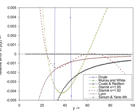
Fig. 1 Relative accuracy of different approximations for the temperature integral. a) overview, b) enlarged view.
Analyses of accuracies of selected approximations of the temperature integral have been published in several works [15,37,38]. Comparison of the accuracies of these approximation is straightforward, and in Fig. 1 the accuracies are compared by plotting pa/p-1. The figure shows that, as expected, the 4th order Senum and Yang approximation is the most accurate of the equations presented above. The two next most accurate approximations are Starink’s approximation for κ = 1.95 and Coats and Redfern’s approximation. The Doyle approximation proves to be the most inaccurate of the ones considered here.
Type B-κ: Direct p(y)-isoconversion methods
[image:9.595.71.527.86.459.2]uses the Murray and White approximation Eq. (19). In general all approximations that are of the form of Eq. (23) lead to a direct p(y)-isoconversion method. Of which the general form is:
3
ln C
RT E A
Tf f
+ −
=
κ
β (26)
So, Doyle’s approximation leads to:
4 0518
. 1
ln C
RT E
f
+ −
=
β (27)
This is the Flynn-Wall-Ozawa method in which the E is determined from the slope of plots of ln(β/Tf 2) versus 1/Tf. Using Eq. (24) the following equation is derived:
5 95
. 1
ln C
RT E
Tf f
+ − =
β (28)
Thus Ea is determined from the slope of plots of ln(β/Tf1.95) versus 1/Tf. And using Eq. (25) we can derive:
6 92
.
1 1.0008
ln C
RT E
Tf f
+ −
=
β (29)
Thus, in this newly derived method, E is determined from the slope of plots of ln(β/Tf1.92) versus 1/Tf.
From the above it is clear that by applying different approximations of p(y) a wide range of direct p(y)-isoconversion methods can be derived. In view of the many possible methods we will classify them as type B-κ isoconversion methods with κ the exponent defined in Eq. (26). Thus the Flynn-Wall-Ozawa method is the Type B-0 method, the Kissinger-Akahira-Sunose (KAS) method is the Type B-2 method and Eqs. (27) and (28) are the Type B-1.95 and Type B-1.92 methods. (Similarly the Boswell method described in [14] is Type B-1.)
one variable. It is here proposed that of the p(y)-isoconversion methods, the type B-1.92 method (Eq. (29)) is to be preferred because it has the best accuracy, combined with a simple application.
Type B-κ(it): Iterative p(y)-isoconversion methods
Apart from the direct isoconversion methods (Type B-κ) described above, there are p(y)-isoconversion methods that make use of a correction procedure, which involves iterative procedures to obtain the activation energy. The best known of these iterative p(y)-isoconversion methods is the procedure described by Flynn [8]. This method uses the Flynn-Wall-Ozawa method to obtain a first estimate of the activation energy. Subsequently the activation energy is corrected by a factor that depends on the average value of y for the data, i.e. the average value of E/RT. The equation for the method is thus:
(
)
R E y B
T d
d
f
) ( 1
ln =− ⎟ ⎠ ⎞ ⎜ ⎝ ⎛
β (30)
where B(y) is the correction function. The method is iterative because B(y) can only be determined by estimating E. The first iteration step will be by taking B(y)=1 or B(y) = 1.05. This method will be classed type B-0(it).
A closely related iterative isoconversion method is the one described by Lyon [16]. This method is based on an approximiation of p(y) using the first term of the expansion Eq. (15), which, after taking the logarithm and taking the derivative with respect to 1/T, yields:
(
)
⎟⎟ ⎠ ⎞ ⎜⎜
⎝ ⎛
+ + + − = ⎟ ⎠ ⎞ ⎜ ⎝
⎛ T y y
T d
d
f
2 2 2
1
lnβ (31)
This is then further approximated by using:
⎟ ⎠ ⎞ ⎜
⎝ ⎛ + − ≅ ⎟⎟ ⎠ ⎞ ⎜⎜
⎝ ⎛
+ + +
− T
R E y
y
T 2
2 2
2 (32)
Thus the method is given by:
(
)
⎟⎟ ⎠ ⎞ ⎜⎜ ⎝ ⎛
+ − = ⎟ ⎠ ⎞ ⎜
⎝ ⎛ + − ≅ ⎟ ⎠ ⎞ ⎜ ⎝
⎛ R y
E T
R E
T d
d
f
2 1 2
1
lnβ (33)
Thus the Lyon method makes two mathematical approximations: first the temperature integral is approximated using the first term in Eq. (15) and then the approximation described in the latter equation (by the ≅ symbol) is made by taking (2+y)-1<<1+y.
Another iterative method is described by the present author in Ref. [15], which uses κ=1.8 and hence should be classed type B-1.8(it). In principle, any number of iterative p(y)-isoconversion methods can be devised, simply by defining a derivate in the form of
(
( )
)
f T d
T d
1 lnβ λ
(with λ a constant equalling about 0 to 2) which approximates E/R and subsequently applying a numerical correction.
Some of these iterative p(y)-isoconversion methods can achieve high accuracies. There are, however, some disadvantages. Firstly, if the first step in the method involves a plot that is based on a low accuracy approximation of p(y), the plot will not be a straight line. This is the case with using the Flynn-Wall-Ozawa plot (ln(β) versus 1/Tf). In such a case it would not be possible to use a deviation of a straight line to determine potential problems in application of the method. For instance, if two thermally activated processes determined if the reaction studied, an accurate direct p(y)-isoconversion method would reveal this by showing a curved plot. A plot of ln(β) versus 1/Tf is curved because of the inaccurate approximation of p(y) involved, and would hence not allow the identification this situation. (Note that type B-1.8(it) method in [15] was optimised to eliminate such drawbacks.) A second drawback of the iterative p(y)-isoconversion methods is the added complexity, which again might serve to obscure potential problems in the application of the method. 2.3 Maximum rate methods (peak methods)
In the methods considered sofar the equivalent stage of the reaction is taken as the stage at which a fixed amount of material has transformed, or where a fixed fraction of the total amount transformed has transformed. Alternatively, it is possible to approximate a fixed stage of the reaction as the stage at which the maximum rate of transformation is achieved, the best know method is the Kissinger method. In several papers [5,23] the validity of this approximation has been investigated by considering mathematical expressions for the reaction function f(α). It was found that the maximum rate of a transformation indeed approximately occurs at a fixed fraction transformed. However, for all considered reaction functions f(α), always small variations in the transformed fraction at maximum reaction rate with heating rate do occur. Thus whilst it is possible to use the maximum reaction rate to define an isoconversion method, a small error will be introduced.
In principle the maximum rate can be used both in type A or type B methods, but due to the popularity of the Kissinger method, it is this type B method that is the dominant method in the maximum rate methods. We will indicate this class of methods by adding the ‘peak’ to the classification symbols, i.e. the Kissinger method is the type B-2-peak method. Type B-1.92-peak and type B-1.95-peak methods are likely to be more accurate than the type B-2-peak method. (But no published applications are known to the present author.) It is further noted that the accuracy of type B-0-peak and type B-1.8-peak(it) methods were investigated in Ref. [23].
2.4 Other Activation Energy analysis methods
Achar-Brindley-Sharp method [41] the Chatterjee method [42] and the temperature criterion method [4,43]. Characteristic of these methods is that they either assume that a particular kinetic model holds or that activation energies can be derived from a single experiment at one single heating rate. These methods have been reviewed by various authors [44,45,46], most recently by Ortega [4], and are found to be generally unreliable, especially for solid-state reactions where the reaction kinetic model is generally complicated, and often unknown.
Further, there are more complex “model free” methods, akin to isoconversion methods, which avoid using an approximation of p(y). The expressions are generally complex and non-linear; and solutions can be obtained using computer algorithms, some of which are available in commercial software. The “model free” non-parametric kinetics (NPK) method derived by Serra and co-workers [47,48] is considered to be accurate, but, due to its mathematical complexity, has been applied very little [1]. (It was shown that for one particular reaction occurring at about y=30, the method obtained an activation energy 0.6% higher than the KAS method. As is shown below that at y=30 the KAS analysis is very accurate, this single example suggests that the NPK method is quite accurate.) The non-linear “model free” isoconversion method by Vyazovkin [27,28] has been applied in commercial software. In the next section, it is shown that a comprehensive analysis of accuracies of the methods described in 3.1 to 3.3 can be made, but this approach is not possible for these computer based methods by Vyazovkin and Serra and co-workers. No detailed analysis of the errors related to these methods is available, apart from the observation that these methods avoid introducing errors related to approximation of p(y). However, as the errors due to approximations of p(y) are small provided an accurate method is selected (see next section) and often smaller than errors introduced by other factors, it is at present not evident that there is a benefit to be gained by applying these complex algorithms for activation energy analysis.
4 Accuracies of isoconversion methods
In order to arrive at recommendations as to which of the many proposed methods for activation energy analysis is most appropriate, the accuracy of these methods needs to be analysed. These accuracies are determined by six factors:
i. Mathematical approximations. Type B isoconversion methods use approximations of the temperature integral. This approximation causes inaccuracies which depend on the type of approximation chosen as well as T and E. The Lyon method additionally uses a further mathematical approximation.
ii. For all methods the temperature at constant amount transformed needs to be obtained from the measured data. This is prone to slight inaccuracies due to limitation in the accuracy of the baseline determination and minor inaccuracies in the measurement of the sample temperature. (This error will be small for maximum rate methods.)
iii. Type A methods require experimental data on reaction rate at constant amount transformed. This data is prone to inaccuracies resulting from a limitation in the accuracy of the baseline determination and in the determination of the temperature at constant amount transformed. iv. Small fluctuations in the supposedly constant heating rate may cause errors in determination
v. In maximum rate methods, the temperature stage defined is not exactly at constant amount transformed, thus introducing small deviations [5,37,49].
vi. All methods presume that the equilibrium state is constant. In some cases this assumption may not hold and this introduces deviations in the measured activation energies [23,50]. The different sources of inaccuracies for various methods are gathered in Table 1.
The deviations introduced by factors v and vi are analysed in some detail elsewhere [5,23,37], and to assess the relative importance of the other factors the following analysis is applied. Consider the activation energy is derived from two constant heating rate experiments, I and II. Then the activation energy for a p(y)-isoconversion method described by Eq. (26) is given by:
II f I f II f II I f I m T T T T R E , , , , 1 1 ln ln − − = κ κ β β (34)
where Em stands for the measured value of E. The deviation, ΔEm, introduced by the different sources of error is approximated as:
int) ( − Δ + Δ ∂ ∂ + Δ ∂ ∂ + Δ ∂ ∂ + Δ ∂ ∂ =
Δ T E E E T
T E T T E
E II m
II m I I m II II m I I m
m β β β β (35)
where the first four terms on the right hand relate to the inaccuracies in determination of the temperatures at fixed fraction transformed and the inaccuracies in determination of heating rate, and ΔE (T int) is the deviation introduced as a result of the approximation made in the T integral, p(y). As the heating rate can generally be determined to a very high accuracy, ΔβI and ΔβII terms in Eq. (35) can be ignored. The first term on the right hand side of the latter equation is evaluated as:
I I m II I II I I m T RT E T T T R T T E Δ ⎟ ⎟ ⎠ ⎞ ⎜ ⎜ ⎝ ⎛ ⎥ ⎦ ⎤ ⎢ ⎣ ⎡ + − = Δ ∂ ∂ κ (36)
As κ <<E/RT we can approximate:
⎟⎟ ⎠ ⎞ ⎜⎜ ⎝ ⎛ − Δ ≅ Δ ∂ ∂ I II II I I m I I m T T T T T E T T E (37)
Thus for type B methods, the errors introduced by error sources i to iv are mostly dominated by error sources i and ii, and the errors can be approximated:
m m II I I II II I II II I I m m E T E T T T T T T T T T T E
E Δ ( −int)
+ − Δ + − Δ ≅ Δ (38)
m m I II II II I I m m E T E T T T T T T E
E Δ ( −int)
+ − Δ + − Δ ≅ Δ (39)
The last term in the latter equation can be determined as follows. From Eqs. (6) and (7) we can derive that for type B methods:
const y p f = ⎟⎟ ⎠ ⎞ ⎜⎜ ⎝ ⎛ β ) ( ln (40)
The general form for the approximation of p is given by )
( )
(y e q y
pa = −y (41)
If the ration between p and the approximation pa is r(y) Eq. (40) can be rearranged to:
(
r y)
const y q y y r y q e y r ypa f y f f
= + ⎟⎟ ⎠ ⎞ ⎜⎜ ⎝ ⎛ + − = ⎟ ⎟ ⎠ ⎞ ⎜ ⎜ ⎝ ⎛ = ⎟⎟ ⎠ ⎞ ⎜⎜ ⎝ ⎛ − ) ( ln ) ( ln ) ( ) ( ln ) ( ) ( ln β β β (42)
and thus it follows
( )
= −( )
(
)
= ⎜⎜⎝⎛ −(
( )
)
⎟⎟⎞⎠ ⎟⎟ ⎠ ⎞ ⎜⎜ ⎝ ⎛ y d y r d R E T d y r d R E T d y q d f ) ( ln 1 1 ) ( ln 1 ) ( ln β (43)Thus we can conclude that:
(
)
( )
d(
( )
y)
p p d y d y r d E T E a mm( −int) = ln ( ) = ln
Δ (44)
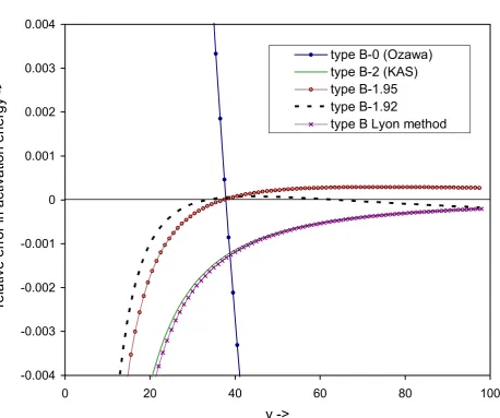
[image:15.595.94.296.71.107.2]The right hand side of the latter equation was evaluated and results are presented in Fig. 2. This figure shows that for the most accurate p(y)-isoconversion method (type B-1.92 method) the deviations introduced by approximation of the temperature integral are less than 0.25% for y>15 and less than 0.75% for y>10. For the Lyon method the sources of error are similar to Type B methods, but in addition an error source related to the approximation in Eq. (32) is introduced. The relative error in E introduced is about -2(y(2+y))-1, and hence accuracy is better than 1.7% for y > 10 and better than 0.8% for y > 15.
[image:15.595.59.503.327.577.2](
)
( )
lim ln( )
( )
0ln lim int)
(
lim 2
≠ ∞
→ = ∞
→ = − Δ
∞ →
−
y d
T d y
y d
p p d y
E T E y
a
m m
κ
(45)
However Fig. 2b shows that deviations are negligible in the range up to y=100, which is the upper limit for realistic y values, provided κ is between about 1.9 and 2.
A rough estimate of deviation introduced by the first two terms on the right hand side of Eq. (39) can be obtained by considering some typical values for solid state reactions ( ≈ 50K with ΔT
≈ 0.25K) and we find that this deviation amounts to about 0.5%. Seeing that for several type B methods the error introduced by approximation of the temperature integral is smaller, the accuracy of the temperature integral approximation has a very limited effect on the overall accuracy of determination of E, provided an accurate type B isoconversion method is used.
II
I T
T −
2a
-0.04 -0.03 -0.02 -0.01 0 0.01 0.02 0.03 0.04
0 20 40 60 80
y ->
re
lat
ive er
ro
r in
ac
tivat
ion en
er
g
y
->
100
type B-0 (Ozawa) type B-2 (KAS) type B-1.95 type B-1.92
2b
-0.004 -0.003 -0.002 -0.001 0 0.001 0.002 0.003 0.004
0 20 40 60 80 100
y ->
rel
a
tive er
ror
in act
ivat
ion ener
gy
->
type B-0 (Ozawa) type B-2 (KAS) type B-1.95 type B-1.92
type B Lyon method
Fig. 2 The fraction error in activation energy caused by approximation of the temperature integral in isoconversion methods type B-0, B-2, B-1.95 and B1.92. For the Lyon method the error due to the approximation in Eq. 32 is given (equalling -2(y(2+y))-1). a) overview, b)
enlarged view.
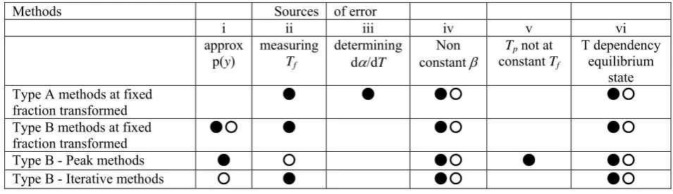
Table 1 Classification of methods.
Description Procedure Type / code Best known / very accurate techniques Ref Rate-isoconversion
method plots of ln(dversus 1/Tαf/dt)
Type A Friedman
Gupta et al [17] [18]
p(y) isoconversion
method plots of ln(Tf κ/β)
versus 1/RTf
Type B-κ Kissinger-Akahira-Sunose (=generalised Kissinger) Ozawa
Type B-1.92
[image:17.595.72.531.78.461.2] [image:17.595.52.563.619.758.2][7,9] [12,13] this paper
Type B - Maximum
rate methods plots of ln(Tp κ/β)
versus 1/RTp
Type B-κ-peak Kissinger [6,7]
Type B - Iterative
methods Type B followed by iterative procedure Type B-κ(it)
Flynn correction of Ozawa method Starink method
Lyon method
The accuracy of the type A methods (rate-isoconversion methods, Friedman method) can be analysed following a similar procedure. For these methods it will hold:
II II m I I m II II m I I m II II m I I m m q q E q q E E E T T E T T E E Δ ∂ ∂ + Δ ∂ ∂ + Δ ∂ ∂ + Δ ∂ ∂ + Δ ∂ ∂ + Δ ∂ ∂ = Δ β β β β (46)
where q= dα/dT. Analysis shows:
II I II II II m II I II I I I m I I II II II I I II I II II II m II I II I I I m I II I I II II I II II I I m m T T T q q E RT T T T q q E RT T T T T T T T T T q q E RT T T T q q E RT T T T T T T T T T T E E − Δ + − Δ + − Δ + − Δ ≅ − Δ + − Δ + − Δ + − Δ ≅ Δ (47)
The first two terms on the right hand side are identical for type A and type B methods, and we may derive a condition which defines in which case a type A method is more accurate than an type B method. The type A method is more accurate if:
m m II I II II II a II I II I I I m I E T E T T T q q E RT T T T q q E
RT Δ ( −int)
< − Δ + − Δ (48)
Seeing that Δq1 and Δq2 are independent we may define a typical accuracy of determination of q, Δq, and rewrite the above condition as:
m m I I II I m E T E T T T RT E dt d dt d q
q ( int)
2
1 − Δ −
< Δ = Δ α α (49)
Accuracy of determination of q may depend on a range of factors including baseline stability and dependency of heat flow calibration on heating rate and temperature, and it is thought that Δq/q may vary between 0.5% and 5% depending on sample and experimental conditions. Considering some typical values for solid-state reactions would yield as indication of the magnitude:
5 . 0 50 500 20 1 = ≈ − I II I I T T T E RT (50)
Choice of activation energy analysis methods
% 1 . 0 ~ < Δ = Δ
dt d
dt d
q q
α α
(51)
Thus if transformation rate can be measured with a precision that is very high (typically better than about 0.1%) type A methods would be more accurate. However, in many cases it will be impossible to guarantee that the rate of transformation can be measured to this accuracy and in these cases the type A methods are not recommended. It should also be considered that it may be very difficult to estimate the accuracy of the determination of Δq, and thus it is very difficult to estimate the possible errors resulting from application of type A methods. In such cases it would be better to accept the limited but quantifiable deviation in type B methods (introduced by the approximation of p(y)) rather than apply a type A method in which the deviations are difficult to quantify.
In summarising the assessment it is thought that for activation energy analysis one of the more accurate type B isoconversion methods is in most cases the most appropriate method.
Table 2 General assessment of the sources or error in methods for activation energy analysis. Black dot means important source of errors, open circle means source of error that is small and usually negligible.
Methods Sources of error
i ii iii iv v vi
approx
p(y)
measuring
Tf
determining
dα/dT
Non
constant β constant Tp not at Tf
T dependency equilibrium
state Type A methods at fixed
fraction transformed z z z| z|
Type B methods at fixed
fraction transformed z| z z| z|
Type B - Peak methods z | z| z z|
Type B - Iterative methods | z z| z|
5 Concluding remarks
[image:19.595.48.526.417.555.2]6 Conclusions
Over the past decades a bewildering range of methods for obtaining the activation energy from experiments at constant heating rate have been proposed. In the present work the isoconversion methods have been classified and their accuracies have been investigated.
• Type A isoconversion methods such as Friedman methods make no mathematical approximations.
• Type B isoconversion methods, such as the generalised Kissinger and Ozawa methods, apply approximations for the temperature integral. Due to the large range of approximations for the temperature integral a wide range of type B methods exist
• Expressions for the accuracies of the type A and B methods are derived.
• The accuracy of the Type B methods proposed in the literature is variable, but highly accurate variants are available. For the more accurate methods identified the approximation of the temperature integral is highly accurate and in practical cases this approximation has virtually no influence on the overall accuracy of the method when applied to real data.
• The Ozawa method is very inaccurate. The accuracy of the Kissinger and generalised Kissinger methods is limited to about 1%. Several lesser known but highly accurate Type B methods are available (accuracy better than 0.5% for y>15), and these are preferred over the better known (generalised) Kissinger and Ozawa methods.
• For real experimental data determination of baselines of the thermal analysis data is never perfect and accuracy of determination of transformation rates is hence limited. In these circumstances type B methods are generally more accurate than type A methods.
References
1 J. D. Sewry and M. E. Brown Thermochim. Acta 390 (2002) 217
2 A.K. Galwey and M.E. Brown, in: M.E. Brown (Ed.), Handbook of Thermal Analysis and Calorimetry, Vol. 1, Elsevier, Amsterdam, 1998, p. 147
3 S. Vyazovkin Thermochim. Acta 355 (2000) 155 4 A. Ortega, Int J. Chem. Kinet. 34 (2002) 193.
5 Xiang Gao, Dun Chen and D. Dollimore, Thermochim. Acta 223 (1993) 75 6 H.E. Kissinger, J. Res. Nat. Bur. Stand. 57 (1956) 217
7 H. E. Kissinger, Analyt. Chem. 29 (1957) 1702 8 J.H. Flynn, J. Thermal Anal. 27 (1983) 95
9 T. Akahira and T. Sunose, Trans. Joint Convention of Four Electrical Institutes, 1969, 246 10 E.J. Mittemeijer, J. Mater. Sci. 27 (1992) 3977
11 H. Flynn and L.A. Wall J. Polym. Sci. 4 (1966), p. 323. 12 T. Ozawa, J. Therm. Anal. 2 (1970) 301
13 T. Ozawa, Thermochim. Acta 203 (1992) 159 14 P.G. Boswell, J. Thermal Anal. 18 (1980) 353 15 M.J. Starink, Thermochim. Acta, 288 (1996) 97 16 R. E. Lyon, Thermochim. Acta, 297 (1997) 117 17 H.L. Friedman, J. Polym. Sci. C, 6 (1964) 183
18 A.K. Gupta, A.K. Jena and M.C. Chaturvedi, Scr. Metall. 22 (1988) 369 19 C.-R. Li and T.B. Tang, Thermochim. Acta 325 (1999) 43
21 L.V. Meisel and P.J. Cote, Acta Metall. 31 (1983) 1053
22 T.P Prasad, S.B. Kanungo and H.S. Ray, Thermochim. Acta 203 (1992) 503 23 M.J. Starink, J. Mater. Sci. 32 (1997) 6505
24 G.R. Heal, Thermochim. Acta 340-341 (1999) 69
25 S. Vyazovkin and V.V. Goriyachko Thermochim. Acta 194 (1992) 221 26 S. Vyazovkin and A.I. Lesnikovich, Russ. J. Phys. Chem. 62 (1988) 2949 27 S. Vyazovkin and D. Dollimore. J. Chem. Inf. Comp. Sci. 36 (1996) 42 28 S. Vyazovkin. J. Therm. Anal. 49 (1997) 1493
29 D.W. Henderson, J. Non-Cryst Solids 30 (1979) 301
30 O. Schlőmilch, Vorlesungen űber hőheren Analysis, 2nd Ed, Braunschweig, 1874, p. 266
31 G.I. Senum and R.T. Yang, J. Thermal Anal. 16 (1977) 1033 32 P. Murray and J. White, Trans. Brot. Ceram. Soc. 54 (1955) 204 33 A.W. Coats and J.P. Redfern. Nature 201 (1964) 68
34 C.D. Doyle, J. Appl. Polym. Sci. 5 (1961) 285 35 C.D. Doyle, J. Appl. Polym. Sci. 6 (1962) 693 36 C.D. Doyle, Nature, 207 (1965) 290
37 J.M. Criado and A. Ortega, J. Non-Cryst. Solids 87 (1986) 302
38 J.W. Graydon, S.J. Thorpe and D.W. Kirk, Acta Metall. Mater. 42 (1994) 3163 39 E.S. Freeman and B Carroll, J. Phys. Chem. 62 (1958) 394.
40 S.M. Ellerstein, in R.S. Porter and J.F. Johnson (Eds.), Analytical Calorimetry, Plenum Press, New York, 1968, 279.
41 B.N.N. Achar, G.W. Brindley and J.H. Sharp, in L. Heller, A. Weiss (Eds.), Proc. Int. Clay Conf., Jerusalem, 1 (1966) 67.
42 P.K. Chatterjee, J. Polym. Sci. A3 (1965) 4253. 43 A. Ortega, Thermochim. Acta 276 (1996) 189
44 J.M. Criado and A. Ortega, J. Thermal Anal. 29 (1984) 1225
45 J.M. Criado, A. Ortega and F. Gotor, Thermochim. Acta 157 (1990) 171 46 S. Vyazovkin and C. A. Wight, Thermochim. Acta 340-341 (1999) 53 47 R. Serra, R. Nomen and J. Sempere, Thermochim. Acta 316 (1998) 37 48 R. Serra, R. Nomen and J. Sempere, J. Therm. Anal. 52 (1998) 933
49 Dun Chen, Xiang Gao and D. Dollimore, Thermochim. Acta 215 (1993) 109