Using the method of weighted residuals to compute potentials of mean force

Using the method of weighted residuals to compute

potentials of mean force

Eric C. Cyr

_{, Stephen D. Bond}

University of Illinois at Urbana-Champaign, Department of Computer Science, Urbana, IL 61801, USA

Received 28 July 2006; received in revised form 19 December 2006; accepted 22 December 2006 Available online 10 January 2007

Abstract

We propose a general framework for approximating the potential of mean force (PMF) along a reaction coordinate in conformational space. This framework, based on the method of weighted residuals, can be viewed as a generalization of thermodynamic integration and direct histogram methods. Using weighted residuals allows for higher-order approxima-tions to the PMF in the form of a global spectral method or a finite element method. In addition, the higher degree of continuity provided by spectral and higher-order elements makes weighted residual methods an attractive choice for use in tandem with biasing force methods. As an analysis tool, the weighted residuals framework provides a context for direct comparison of thermodynamic integration and histogram based methods. For validation of the new method, numerical experiments are performed on two systems: a simple double-well and alanine dipeptide in vacuum. Comparisons between the new weighted residual methods, thermodynamic integration, and WHAM are performed. When configuration space is perfectly sampled the high-order weighted residual methods are found to exhibit exponential convergence. For more realistic sampling, the weighted residual methods performed comparably to the other two. However, results suggest that spectral type methods are more robust with respect to parameter choices describing the solution space.

Ó2007 Elsevier Inc. All rights reserved.

Keywords: Potential of mean force; Method of weighted residuals; Free energy; Thermodynamic integration; Histogram methods

1. Introduction

The potential of mean force (PMF) is one of the most important concepts in physical and biological chem-istry[1]. It describes the change in free energy along a ‘‘reaction coordinate’’ and determines the strength and likelihood of association in molecular systems[2]. Estimating the change in free energy between two molecular conformations is a challenging task due to the high dimensionality of phase space and complex structure of the energy landscape[3].

A variety of techniques have been developed to approximate the PMF including umbrella sampling[4], weighted histograms [5], free energy perturbation [6,7], thermodynamic integration[7,8], steered molecular

0021-9991/$ - see front matter Ó2007 Elsevier Inc. All rights reserved. doi:10.1016/j.jcp.2006.12.015

* _{Corresponding author.}

E-mail addresses:[email protected](E.C. Cyr),[email protected](S.D. Bond).

dynamics[9]and adaptive biasing forces[10–13]. These methods sample configuration space using a sequence of (biased) equilibrium or nonequilibrium molecular dynamics or Monte Carlo simulations. The PMF is recovered using either the observed probability density or mean force.

In this paper we propose a novel framework for the approximation of the PMF along a reaction coordinate from configurations generated by molecular dynamics and Monte Carlo simulations. This framework, based on the method of weighted residuals, allows for the comparison of a wide class of existing free energy methods and provides a platform for deriving new methods.

Comparisons between free energy methods have been performed in the past. Both[14,15]found that ther-modynamic integration (TI) was slightly superior to free energy perturbation (FEP). In a study comparing the use of the weighted histogram analysis method (WHAM), TI and FEP to compute solvation free energies, WHAM was found to perform better than TI and FEP [16]. Recently the adaptive biasing force (ABF) method was favorably compared to a method based on Jarzynski’s identity [12].

The structure for the remainder of this paper is as follows. In Section2, we define the potential of mean force in terms of the underlying probability density function. Direct histogram, thermodynamic integration and umbrella sampling methods are reviewed in Section3. Weighted residuals methods are introduced in Sec-tion3.4, where it is shown that direct histogram and thermodynamic integration methods are both weighted residuals methods. This framework is used to develop two new methods based on Chebyshev polynomials and spectral elements. Analytical results using a simple model problem indicate that the weighted residual methods are more accurate when conformational space is well sampled. To investigate sampling sensitivity, a sequence of numerical experiments are conducted in Section4. Results indicate that the new weighted residual methods are competitive and more robust with respect to parameter choices.

2. Potential of mean force

The potential of mean force (PMF) is the free energy along a reaction coordinate (or path) in conforma-tional space. The reaction coordinate, denoted byn(x), is a function which maps atomic positions,x, to a con-tinuous collection of states, n(x). A specific state, f, is the set of atomic positions for which nðxÞ ¼f. The reduced probability density function corresponding to the state fis given by

qnðfÞ ¼

Z

dðnðxÞ fÞqðx;pÞdxdp; ð1Þ

wherex is the atomic positions,p is the momenta, andqðx;pÞis the probability density function associated with the ensemble. In this paper we assume conformations are sampled from the constant temperature or canonical ensemble,

qðx;pÞ ¼ e bHðx;pÞ

R

ebHðx0_;p0_Þ

dx0_dp0:

Here Hðx;pÞ is the Hamiltonian of the system, the sum of the potential and kinetic energy terms, and

b¼1=kBT, wherekB is the Boltzmann constant and T is temperature. The PMF, A(f), is defined in terms

of the relative probability density at a statefby

AðfÞ ¼ 1 b ln

qnðfÞ qnðf0Þ

; ð2Þ

wheref0is the reference state which can be chosen arbitrarily. Note that the PMF is defined up to an additive

constant depending on the reference state. For a finite range of states,½fa;fb, the reference state is often set to fain which case the resulting PMF atfbis the change in free energy between statesfaandfb.

The mean force can be written as an ensemble average using the derivative of the PMF (see[12,13]). Dif-ferentiating Eq.(2)with respect tofresults in

dAðfÞ

df ¼

oH

of

f

¼ hFnif ¼

R

Fnðx;pÞdðnðxÞ fÞqðx;pÞdxdp

R

wherehifdenotes the average atnðxÞ ¼f[12,13]. The averagehFnifis the mean force acting in the direction of

the reaction coordinate. Here, Fnðx;pÞis a function of atomic positions and momenta. The analytical form

used in this paper is

Fnðx;pÞ ¼

2

b

rnðxÞTM1_n00_ðxÞM1_rnðxÞ

ZnðxÞ

2

rUðxÞTM1_rnðxÞ

ZnðxÞ

þp

T_M1_n00_ðxÞM1_p

ZnðxÞ

; ð4Þ

whereMis the mass matrix,Uis the potential energy andZn¼ rnTM1rn. The derivation of Eq.(4)can be

found in[11]. Additional forms can also be found in[17,10], however, they are more cumbersome then Eq.(4)

because they require a coordinate system orthogonal ton to be defined. A convenient representation of the mean force is the ratio of two ensemble averages,

hFnif¼

FnðfÞ

q_nðfÞ: ð5Þ

Here,FnðfÞ, is defined as the numerator of Eq.(3)

FnðfÞ ¼

Z

Fnðx;pÞdðnðxÞ fÞqðx;pÞdxdp:

3. Numerical methods

In this section we present numerical methods for approximating the PMF. We start by reviewing existing direct histogram and thermodynamic integration (TI) methods before introducing the weighted residuals method. Using the weighted residuals framework we show that the direct histogram and TI methods are sim-ilar in that they both treat the approximation to the PMF as a linear combination of basis functions along the reaction coordinate

AðfÞ X

N

i¼1

Ai/iðfÞ:

The methods only differ in the choice of basis functions,/i, and formula for computing the coefficients,Ai.

Each coefficient is a single degree of freedom describing the approximation, in this case the approximation hasNdegrees of freedom (DOF). To illustrate the flexibility of weighted residuals, we apply two new methods based on Chebyshev polynomials and spectral elements.

Without sufficient sampling of conformational space, none of the methods described in this paper can accu-rately reconstruct the PMF. In regions whereq_nðfÞis small, the sampling will be poor due to high potential barriers. Effective removal of these barriers can be difficult since it generally requires knowledge of the under-lying PMF. One biasing method, known as umbrella sampling, uses a restraining potential to increase sam-pling in a region of interest. In Section 3.3, we review umbrella sampling and the weighted histogram analysis method (WHAM) for combining data from a sequence of biased simulations.

3.1. Direct histogram method

The direct method calculates the probability distribution simply by building a histogram using binning. Binning requires breaking up the reaction coordinate into intervals or bins and then counting the number of times a molecular dynamics (MD) or Monte Carlo (MC) simulation reaches each bin. This gives a histo-gram from which a piecewise-constant representation of the probability density functionqnðfÞcan be found.

The coefficients in this expansion are calculated by

Pi¼ 1

D

Z

/_iðnðxÞÞqðx;pÞdxdp¼1 D

Z D=2

D=2

q_nðfiþfÞdf; ð6Þ

^ qnðfÞ ¼

XN

i¼1

Pi/iðfÞ:

Note in the limit as D!0 the approximation^qnðfÞ !qnðfÞ. To find the PMF, the approximate probability

density function,q^nðfÞ, is inserted into Eq.(2) resulting in

AðfÞ 1 b ln

XN

i¼0

Pi P0

/iðfÞ !

¼X

N

i¼0

1

bln

Pi P0

/iðfÞ ¼

XN

i¼0

Ai/iðfÞ:

The summation commutes with the logarithm only in the case that/iis piecewise-constant. This would not be possible if/iwere a higher-order polynomial.

There are two forms of error arising from this approximation, statistical and truncation error. Statistical error comes from using a finite sample size to approximate an average. This error decreases as Dincreases. The truncation (or systematic) error is a result of approximating a delta function with 1

D/i. To see this, con-sider Eq.(6). The coefficientPiis also an approximation ofqnðfiÞ, wherePiandqnðfiÞcan be written as the ensemble average of1

D/ianddrespectively. They are equivalent in the limit asD!0; however, for nonzeroD, a truncation error is made. Therefore the truncation error decreases asDdecreases, which is in opposition to the statistical error. In the absence of statistical error, the total error will be equal to the error from a piece-wise-constant approximation of the PMF. A complete discussion of these errors and how to balance the two can be found in [18].

3.2. Thermodynamic integration

Thermodynamic integration (TI) relies on Eq.(3) to compute the mean force. Once computed, the mean force is integrated along the reaction coordinate to recover the PMF

AðfÞ ¼

Z f

f0

hFnifdf:

hFnifcan be calculated from a constrained MD or MC simulation[19]; however, doing so suffers from

prob-lems due to non-ergodic sampling. Regions normally accessible may become blocked by high potentials per-pendicular to the reaction coordinate. Consequently the configuration space is not adequately sampled in finite simulation time [13].

A second option for computinghFnif is to use an unconstrained simulation in which the system is allowed

to move freely, both in the direction of the reaction coordinate and in perpendicular directions. In this paper TI is assumed to be unconstrained unless otherwise stated. From an implementation perspective TI uses bin-ning similarly to the direct method. The reaction coordinate is broken up into bins and, over the course of an MD or MC simulation, values ofFnðx;pÞare recorded in each bin. In post processing, the bin averages are

computed yielding an approximation of hFnif. Similar to the direct method, the mean force calculated by

TI yields a piecewise-constant approximation to hFnif. The coefficients in this expansion are

Fi¼ RD=2

D=2FnðfiþfÞdf RD=2

D=2qnðfiþfÞdf

: ð7Þ

In terms of /i, a unit constant basis function with support over the bin defined by the intervalfiD=2, the approximation ofhFnif at any value of the reaction coordinate is written as

hFnif

XN

i¼1

Fi/iðfÞ:

Integrating results in

AðfÞ

Z f

f0

XN

i¼1

Fi/iðf0Þdf0¼

XN

i¼1

Fi

Z f

f0

which implies that TI provides a piecewise-linear approximation of the PMF. The coefficients suffer from the same type of statistical and truncation error as the coefficients for the direct method. For perfect sampling (no statistical error) the error in the TI approximation will be equal to the error from a piecewise-linear approx-imation of the PMF. For this reason, if the PMF is smooth and the bin sizes are the same, the TI approxi-mation will be better then the direct histogram approxiapproxi-mation in the absence of statistical error.

Recently Darve et al.[10–12]proposed a TI method that uses the most recent estimate of the PMF to bias the simulation. This method is known as the adaptive biasing force (ABF) method. Continuously updating the biasing potential with the best estimate of the PMF allows for eventual convergence to uniform sampling along the reaction coordinate, which leads to better sampling and faster convergence to the PMF. A descrip-tion of an implementadescrip-tion of ABF and its details can be found in[13].

3.3. Umbrella sampling

The problem of poor sampling in unlikely regions of configuration space is present in both TI and the direct method. One way to alleviate this problem is through umbrella sampling, originally described in[4]. The idea is to run several simulations/trajectories with sampling that is restricted to a small portion of the reaction coordinate using a (typically quadratic) restraint potential. Ensemble averages calculated in separate trajecto-ries can be recombined to give the desired average (see[4,20]). It is also possible to reduce barriers along the reaction coordinate by applying a bias that is the negative of an estimate of the PMF. The removal of this bias is the same as for the restraint potentials.

When calculating the PMF with the TI method, the restraint potentials allow adequate sampling along the reaction coordinate over the domain of interest. Since the restraint potential depends only on the reaction coordinate, the sampling perpendicular to the reaction coordinate is not changed by the bias. Therefore, the averagehFnif is unaffected by the bias and no re-weighting is required when recombining the samples.

For direct methods, the effects of the biasing potential must be removed from the resulting biased histo-gram. One of the most popular methods for bias removal is the weighted histogram analysis method (WHAM)

[5], which employs a specific choice of weights to combine the averages. Briefly, ifqi

nðfÞis an average

calcu-lated from theith ofTtrajectories thenqnðfÞcan be calculated as

qnðfÞ ¼

XT

i¼1

wiðfÞqinðfÞ; where

XT

i¼1

wiðfÞ ¼1 8f:

The weights are chosen to minimize the variance inqnðfÞ. For more details, see[21,22].

3.4. Method of weighted residuals

The method of weighted residuals is a technique used to find approximate solutions to ordinary and partial differential equations of the form

LuðxÞ ¼fðxÞ for x2X; ð9Þ

whereLis a differential operator andXis the domain of the problem. The approximate solution,^u, is repre-sented as a linear combination ofNbasis functions/iwhose span forms the trial space. The coefficients are determined by forcing the residual,rðxÞ ¼L^uðxÞ fðxÞ, to be orthogonal to a test space spanned byNbasis functionswj. Enforcing orthogonality yields a set of Nequations to be solved for Nunknown coefficients

Z

X

wjðxÞrðxÞwðxÞdx¼0 for j¼1;. . .;N;

wherew(x) is a strictly positive weight function. In the case thatLis a linear operator, the resulting system of equations will also be linear.

squares is also a weighted residual method withw_j¼or=ouj, whereuiare the unknown trial space coefficients [23].

The weighted residuals approximation to the PMF can be found using the residual defined by Eq. (3). Using the uniform weight function, wðfÞ ¼1, and the test functionsfwig

N

i¼1 gives theNequations

Z ff

f0

oA

ofþ hFnif

w_jðfÞdf¼0 forj¼1;. . .;N:

A difficulty of this formulation is that to integrate hFnifwiðfÞrequires hFnif to be evaluated at quadrature

points. Each evaluation is subject to both truncation and statistical error. This problem can be avoided if the weight function is chosen to bewðfÞ ¼qnðfÞ, which results in the new set of equations

Z ff

f0

oA

ofþ hFnif

wjðfÞqnðfÞdf¼0 for j¼1;. . .;N: ð10Þ

Substituting the trial basis functionsf/ig N

i¼1 and simplifying Eq.(10)by applying Eq.(5) gives

Z ff

f0

dA dfþ hFnif

w_jðfÞqnðfÞdf¼0

)

Z ff

f0

dA

dfwjðfÞqnðfÞdf¼

Z ff

f0

hFnifwjðfÞqnðfÞdf

)X

N

i¼1

Ai Z ff

f0

/0_iðfÞwjðfÞqnðfÞdf¼

Z ff

f0

FnðfÞwjðfÞdf:

Notice the integrals in the last expression are ensemble averages. This further simplifies the system (assuming

/iandwjhave support only on½f0;ff) to give

XN

i¼1

Aih/0iðnðxÞÞwjðnðxÞÞi ¼ hFnðx;pÞwjðnðxÞÞi forj¼1;. . .;N; ð11Þ

wherehidenotes the ensemble average over all of configuration space.

With an appropriate choice of basis functions it is possible to derive the TI method from the weighted resid-ual framework. Define a grid such thatfi¼f0þ i12

Dfori¼1;. . .;N, wherefN þD=2¼ff. Now define the derivative of the basis function /i to be 1 on the intervalfiD=2 and zero otherwise. Note these basis functions are the same as the basis functions used to approximate AðfÞin TI (see Eq. (8)). They will make up the trial space in a weighted residual method. Using a least squares approach the test space will be spanned by/0_j. Substituting the /0_jforwjin Eq.(11)results in

XN

i¼1

Aih/0iðnðxÞÞ/ 0

jðnðxÞÞi ¼ hFnðx;pÞ/0jðnðxÞÞi

)Ajh/0jðnðxÞÞ/ 0

jðnðxÞÞi ¼ hFnðx;pÞ/0jðnðxÞÞi

)Aj¼

hFnðx;pÞ/0jðnðxÞÞi

h/0jðnðxÞÞ/ 0 jðnðxÞÞi

¼

RD=2

D=2FnðfjþfÞdf RD=2

D=2qnðfjþfÞdf

¼ Fj

forj¼1;. . .;N. The last step holds because the function/0_jhas support only on the intervalfiD=2. Notice the coefficientsAjare the negatives of theFicoefficients used by TI in Eq.(7). Hence, the weighted residuals

method with a piecewise-linear trial space and a piecewise-constant test space is the same as TI.

Both TI and the direct method correspond to low-order finite element methods. The systematic error of these methods can be decreased by increasing the number of intervals in the approximation, this process is referred to ash-refinement and yields algebraic convergence. It is possible when using Eq.(10)to use high-order finite elements so-called spectral element methods (SEM) or even global spectral methods (GSM). High-order approximations have greater smoothness and can also take advantage of the exponential conver-gence coming from increasing the order of the approximation, referred to asp-refinement. Hybrid methods that use both forms of refinement are possible, SEM is particularly well suited to this approach[23,24].

As an example, consider the double well potential

Uðx;yÞ ¼2ðyx3_þxÞ2 þ1

4x

4_þex2

: ð12Þ

If we let the reaction coordinate be defined asnðx;yÞ ¼x, then the PMF up to an additive constant,C, is

AðxÞ ¼1

4x

4_þ

ex2þC: ð13Þ

Under the assumption of perfect sampling (i.e. no statistical error), the application of Eq.(10)on the interval [1.5, 1.5] leads to the convergence inL2with respect to the degrees of freedom seen inFig. 2. Here the GSM uses Chebyshev polynomials, refining solely inp, resulting in rapid exponential convergence. The steps in the curve are due to the even-degree of the exact solution since the addition of odd-degree basis functions does not improve the approximation. The SEM shows similar rapid convergence due top-refinement. Here the number of elements is held fixed at 50 while each element is refined inp. Finally, TI uses fixed-degree piecewise-linear elements combined with pureh-refinement.

In addition to the rapid theoretical convergence and greater smoothness of higher-order approximations,p -refinement also reduces the statistical error associated with small bin sizes. For a SEM, the bin (or element size) can remain fixed while the degree is increased. Alternatively, if a GSM is used there will be no sampling

Fig. 1. A table showing the test and trial spaces used by thermodynamic integration and the direct method, with respect to the weighted residuals described by Eq.(10).

10–0 10–1 10–2 10–3

10–16 10–14 10–12 10–10 10–8 10–6 10–4 10–2

Degrees of Freedom

L

2 Error

GSM TI SEM

Fig. 2. Loglog plot of theL2_{error of solutions versus the degrees of freedom for the double well potential with the assumption of perfect}

error resulting from using a small bin size. This is not to say that statistical error will no longer exist, it just won’t be connected to bin size.

3.4.1. Multiple biased simulations

The method described by Eq.(11)assumes that samples are coming from an unbiased simulation. However, as discussed in Section3.3, better sampling can be achieved by using several biased trajectories. To apply Eq.

(11), the averages must be computed from a recombination of the biased trajectories. One possible way to do this is to use WHAM. Another approach requires a different choice for the weighting functionw(f). Letukbe

the biasing potential for thekth ofKbiased trajectories. We will choose the weighting function

wðfÞ ¼X

K

k¼1

R

dðnðxÞ fÞebðHðx;pÞþukðnðxÞÞÞ_dxdp R

ebðHðx;pÞþukðnðxÞÞÞdxdp : ð14Þ

When substituted into Eq. (10) with trial functions/i and test functions wj, this choice of weight function yields the system of equations

XN

i¼1

Ai

XK

k¼1

h/0_iðnðxÞÞwjðnðxÞÞi k

¼ X

K

k¼1

hFnðx;pÞwjðnðxÞÞi k

ð15Þ

forj¼1;. . .;N, wherehik is the average coming from thekth biased trajectory. A derivation of Eq.(15)can be found in Section A.2. Notice that the components of the linear system produced by Eq. (15)are simple averages of the biased simulations. No explicit recombination step is necessary to compute the PMF using the weighted residual method.

4. Numerical experiments

To compare the methods for computing the PMF we performed a sequence of numerical experiments on two different systems. The first is the simple double well problem described in Section3.4. The second is ala-nine dipeptide with the PMF computed along the/dihedral angle. Two different error metrics were used to compare the quality of the approximation,A, with the exact PMF,b A. These metrics measure the total error, the sum of the statistical and truncation error, made by the approximation. Recall that the PMF is defined up to an additive constant. We define the first metric to be the L2error minimized with respect to this constant

kAbAkL2¼min a

Z b

a

ððAbðfÞ þaÞ AðfÞÞ2df

1=2

:

The second error metric, referred to as the difference error, measures the error in the change in free energy between two states. The difference error is defined at a pair of points on the interval of interest,f1;f22 ½a;b

jAbAj_D¼ jðAbðf2Þ Abðf1ÞÞ ðAðf2Þ Aðf1ÞÞj:

The number of degrees of freedom (DOF) in the solution space used by TI, the direct method and WHAM is simply the number of elements or bins. For SEM and GSM the DOF is the number of coefficients used in the approximation to the PMF. To solve the WHAM equations, we used a fixed-point iteration with a tolerance of 103using the method described in [21,22]. Further refinement did not have a significant effect on the re-sults. To investigate bothhandp-refinement, we applied the weighted residuals method using GSM and SEM. The basis functions for the global spectral method were constructed using

/iðxÞ ¼

Z x

f0

Ti

2x0_f f f0 ff f0

dx0;

whereTiis theithChebyshev polynomial and refinement is carried out only inp. In the figures, global spectral

4.1. Double well PMF

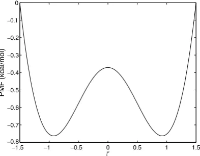
For our first numerical experiment, we considered the simple double well system described in Section3.4. The potential and corresponding PMF can be found in Eqs.(12) and (13). We used the reaction coordinate

nðx;yÞ ¼x, on the interval [1.5, 1.5]. A plot of the exact PMF can be seen inFig. 3. Sampling was done using the Metropolis Monte Carlo algorithm described in[20], withb¼2, and an acceptance ratio of 35%. The sim-plicity of the two-dimensional configuration space made it possible to adequately sample the whole interval with a single unbiased simulation. When computing the difference error we used two critical points,

fl 0:923 andfr¼0, which correspond to the bottom and peak of one well.

TheL2error as a function of the number of DOF is plotted inFig. 4with each plot corresponding to a different simulation length, 3:33103 samples on the left and 3:33105 samples on the right. Refinement for TI and the direct method is performed in h and both GSM and SEM refine inp. Notice in both plots the error of the direct method decreases until an optimal bin width is reached where statistical error is in bal-ance with the truncation error, then increases as statistical error dominates. The remaining methods, all based on the weighted residual method, appear to level off for large degrees of freedom. For the plot with 3:33105

samples, the global spectral method (denoted ‘‘GSM’’) initially achieves very rapid convergence similar to the

–1.5 –1 –0.5 0 0.5 1 1.5

–0.8

–0.7

–0.6

–0.5

–0.4

–0.3

–0.2

–0.1

0

ζ

PMF (kcal/mol)

Fig. 3. Exact PMF for the potential from Eq.(12).

100 101 102 103

10–2 10–1 100

Degrees of Freedom

L

2 Error

3.33× 103 Samples

TI Direct GSM SEM

100 101 102 103

10–3 10–2 10–1 100

Degrees of Freedom

L

2 Error

3.33×105 Samples

TI Direct GSM SEM

Fig. 4. Loglog plot of theL2_{error versus the DOF for the PMF of the double well potential in(12). Notice the direct method has a clear}

minimum after both 3:33103_{samples and 3}

exponential convergence seen in Fig. 2. However, the curve levels when the statistical error begins to domi-nate. Also notice the direct method with optimal bin width achieves higher accuracy then the other methods for both numbers of samples. A similar pair of plots showing the difference error can be seen inFig. 5. Again the direct method has a clearly optimal bin width. An interesting difference is that GSM has an error that is an order of magnitude less than the smallest error achieved by the remaining methods for fewer degrees of freedom.

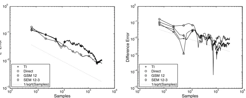
Fig. 6shows theL2and difference errors as functions of the number of samples for the four different

meth-ods. The TI and direct methods both have 50 degrees of freedom. The spectral element method (SEM) uses 12 elements with a cubic polynomial basis. Finally GSM is implemented with a degree 12 Chebyshev basis. The final line on the plots serves as a reference for 1=pffiffiffiffiN, whereNis the number of samples. The plot shows that all methods are converging in both norms as 1=pffiffiffiffiN. In theL2plot all the methods have very similar error, the notable exception being the direct method. The direct method does not appear to do as well with the difference error over the entire length of the simulation. The remaining three methods again have very similar performance.

100 101 102 103

10–3 10–2 10–1 100

Degrees of Freedom

Difference Error

3.33× 103 Samples

TI Direct GSM SEM

100 101 102 103

10–5 10–4 10–3 10–2 10–1 100

Degrees of Freedom

Difference Error

3.33× 105 Samples

TI Direct GSM SEM

Fig. 5. Loglog plot of the difference error versus the DOF for the PMF of the double well potential in(12). On the left is the result after 3:33103_{samples, and on the right is after 3:33}

105_samples.

102 103 104 105 106

10–3 10–2 10–1 100

Samples

L

2 Error

TI Direct GSM 12 SEM 12-3 1/sqrt(Samples)

102 103 104 105 106

10–5 10–4 10–3 10–2 10–1 100

Samples

Difference Error

TI Direct GSM 12 SEM 12-3 1/sqrt(Samples)

Fig. 6. L2_{error (on the left) and difference error (on the right) in the approximation to the PMF of the double well potential as a function}

4.2. Alanine dipeptide

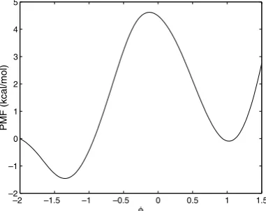
To further examine the performance of the weighted residual methods a more realistic system was studied. Alanine dipeptide was chosen because it shares many of the characteristics of more complex biomolecules[25]. Furthermore, its small size reduces the computational effort required allowing for a more detailed comparison of numerical methods. All simulations were performed on a single workstation using the NAMD software program developed by the Theoretical and Computational Biophysics Group in the Beckman Institute for Advanced Science and Technology at the University of Illinois at Urbana-Champaign[26]. Each simulation generated configurations using Langevin dynamics in vacuum with 1 fs timesteps. The reaction coordinate under consideration was the/dihedral angle measured in radians with [2.0, 1.5] being the interval of interest. The PMF from a 40 ns ABF simulation (shown inFig. 7) was used as the ‘‘exact’’ PMF when calculating errors.

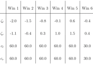
In the double well problem it was possible to sample the entire reaction coordinate using a single unbiased window. For this problem multiple windows had to be used. Initially, five evenly spaced overlapping windows of the same size were chosen to cover the reaction coordinate over the domain. This choice led to poor sam-pling surrounding the maxima of the PMF at / 0:13. An additional window focusing sampling in this region fixed the problem. Sampling was constrained to each window by piecewise-quadratic biasing potentials of the form

uðfÞ ¼ 1

2clðfflÞ

2

f<fl; 0 fl6f6fr;

1

2crðffrÞ

2

fr<f; 8

> < > :

wherecl,crare coefficients controlling the strength of the restraint, andfl,frare positions that define the size

and placement of the window. A table listing the restraints and positions defining the six windows used can be seen inFig. 8. Because of the use of multiple windows, WHAM was used instead of the direct method. Each window was run for a total of 2 ns or 2106time steps, yielding a total simulation time of 12 ns.

Fig. 9shows theL2error as a function of DOF for different types of refinement. On the left is a snapshot

after 0.75 ns of simulation and on the right is the full 12 ns of simulation. Bothhandprefinement were inves-tigated, using a static 8 elements forp-refinement (SEM-p) and cubic polynomials forh-refinement (SEM-h). Notice the error decreases with increased simulation time. In general the error is proportional to 1=pffiffit, wheret

is the length of the simulation. As with the double well potential, all the methods improve until the statistical error overwhelms the truncation error. Unlike the direct method for the double well potential, WHAM does not have an obvious optimal point where the statistical error balances with the truncation error. WHAM instead has a constant error for large numbers of degrees of freedom. The global spectral method again has very rapid convergence for small degrees of freedom, and is superior in the full 12 ns error calculation.

–2 –1.5 –1 –0.5 0 0.5 1 1.5 –2

–1 0 1 2 3 4 5

φ

PMF (kcal/mol)

Fig. 10is similar toFig. 9but uses the difference error defined at the points/¼ 0:13 and/¼1:03. Using this error metric both the h and p-refined SEM methods perform better than suggested by the L2metric. Though the global spectral method is still superior for the total simulation time of 12 ns.

100 101 102 103

100

Degrees of Freedom

L

2 Error

0.75ns of Simulation Time

TI GSM SEM-p SEM-h WHAM

100 101 102 103

102 101 100 101

Degrees of Freedom

L

2 Error

12ns of Simulation time

TI GSM SEM-p SEM-h WHAM

Fig. 9. Loglog plot of theL2error in the PMF for alanine dipeptide as a function of the DOF for 0.75 ns (on the left) and 12 ns (on the right) of total simulation time.

Fig. 8. Windows used when computing the PMF for alanine dipeptide.

100 101 102 103

10–2 10–1 100 101

Degrees of Freedom

Difference Error

0.75ns of Simulation Time

TI GSM SEM-p SEM-h WHAM

100 101 102 103

10–3 10–2 10–1 100

101 12ns of Simulation Time

Degrees of Freedom

Difference Error

TI GSM SEM-p SEM-h WHAM

5. Conclusion

We have developed a framework based on the method of weighted residuals for approximating the poten-tial of mean force (PMF) along a reaction coordinate. This framework is general enough to encompass ther-modynamic integration and direct histogram methods, providing an analysis tool for comparing the two. In addition, using weighted residuals allows for higher-order approximations to the PMF in the form of a global spectral method or a spectral element method. When implemented, the result is a linear system of equations for determining the unknown PMF from ensemble averages generated by equilibrium molecular dynamics or Monte Carlo simulations. We have shown that this holds true even when multiple biased trajectories are used. In our analysis, we have demonstrated that higher-order methods allow for exponential convergence through

p-refinement when configurational space is sampled sufficiently well. For fewer samples statistical error dom-inates and is governed by the law of large numbers, which is proportional to 1=pffiffiffiffiN, whereNis the number of samples. In numerical experiments involving a double-well potential and alanine dipeptide, we have shown that the global spectral method is remarkably robust as the polynomial degree is increased. When the sampling rate was high and the polynomial degree was low, the global spectral method retained its exponential conver-gence rate. As the polynomial degree was increased and statistical error dominated, the total accuracy remained nearly constant. This is in contrast to histogram methods which suffer from increased statistical error as the bin size is refined. Finally, the higher degree of continuity provided by spectral methods makes weighted residuals an attractive choice for use in conjunction with biasing force methods.

Acknowledgments

The authors would like to thank Prof. Robert Skeel for many helpful and stimulating discussions, and the reviewers for their insightful comments.

Appendix A

A.1. Direct methods as weighted residuals

In this section reaction coordinates will have two classifications, first aperiodic reaction coordinates which assumes that at somef0andff, withf0<ff, the system is restrained, i.e.qnðf0Þ ¼qnðffÞ ¼0. Notice that this includes infinite reaction coordinates. The second classification is a periodic reaction coordinate, which is defined byf0¼ff andqnðf0Þ ¼qnðffÞ.

A.1.1. Aperiodic reaction coordinate

First consider the weighted residual method defined by Eq.(10). UsingqnðfÞ ¼ebAðfÞ, notice

bqnðfÞ

dA dfþ hFnif

¼ d

df½qnðfÞ bFnðfÞ:

Multiplying Eq.(10)byband substituting the above expression gives the set of Nequations Z ff

f0

d

df½qnðfÞ bFnðfÞ

w_jðfÞdf¼0 for j¼1;. . .;N:

Now approximateqnðfÞas a linear combination of the trial functionsf/ig N

i¼1. Substituting in the

approxima-tion gives the linear system

XN

i¼1

Pi Z ff

f0

/0_iðfÞwjðfÞdf¼ Z ff

f0

bFnðfÞwjðfÞdf forj¼1;. . .;N:

After first substitutingbFnðfÞ ¼_dd_f½qnðfÞand then integrating by parts on both sides we find

XN

i¼1

Pi ð/iðfÞwjðfÞj ff

f0

h

Z ff

f0

/iðfÞw 0

jðfÞdf ¼ Z ff

f0

qnðfÞw 0

where the boundary terms vanish on the right-hand-side because of the assumption that the reaction coordi-nate is restrained (q_nðf0Þ ¼qnðffÞ ¼0).

Choose a set ofDspaced grid points on the intervalðf0;ffÞ, wheref1>f0þD=2 andfN <ff D=2. The objective is to approximate qnðfÞ on this grid, to this end we will use as trial functions the basis /iðfÞ for i¼1;. . .;N, where

/_iðfÞ ¼ 1 fiD=26f6fiþD=2;

0 otherwise:

ðA:2Þ

The choice of grid points and basis functions enforces that the piecewise-constant approximation toqnðfÞwill

be zero atf0andff. If we require that a functionwiin the test space satisfiesw0iðfÞ ¼/iðfÞand substitute the definitions of/iandwjinto Eq.(A.1)we find

Pj¼ 1

D

Z D=2

D=2

qnðfjþfÞdf forj¼1;. . .;N:

Therefore the coefficients ofPias calculated by this weighted residual method are equivalent to the coefficients

calculated by the direct method (see Eq.(6)). Since the trial space is piecewise-constant, the direct method is the same as applying the weighted residuals method defined by Eq.(10)with the same trial space, and a piece-wise-linear test space.

A.1.2. Periodic reaction coordinate

Define the pointsf0¼f1;. . .;fN ¼ff and use/iðfÞfrom Eq.(A.2)fori¼2;. . .;N1. Fori¼1 define/i as

/1ðfÞ ¼

1 f16f6f1þD=2;

1 fND=26f6fN; 0 otherwise:

8 > < > :

Notice that for i¼1;. . .;N1 the functions /iðfÞ are periodic on ½f0;ff. Now assume that wjðfÞ for j¼1;. . .;N1 are periodic test functions. Repeating the same steps for the weighted residual method as above in the aperiodic reaction coordinate example gives

XN1

i¼1

Pi ð/iðfÞwjðfÞj ff

f0

h

Z ff

f0

/iðfÞw 0

jðfÞdf ¼ ðqnðfÞwjðfÞj ff

f0

Z ff

f0

qnðfÞw 0 jðfÞdf

:

Using the periodicity of/iðfÞ,wjðfÞ,qnðfÞand applying the definition of/iðfÞyields

XN1

i¼1

Pi Z D=2

D=2

w0_jðfiþfÞdf¼ Z ff

f0

qnðfÞw 0 jðfÞdf:

Now let w0_jðfÞ ¼/jðfÞ. For wjðfÞ to be periodic it has to be 0 everywhere but on the interval

½fjD=2;fjþD=2where the function is linear fromwjðfjD=2Þ ¼0 towjðfjþD=2Þ ¼D. The specific form is

wjðfÞ ¼

0 f<fjD=2;

f ðfjD=2Þ fjD=26f6fjþD=2; 0 f>fjþD=2:

8 > < > :

This set of test functions,wjðfÞforj¼1;. . .;N1 gives the same values computed by the direct method for the coefficientsPj.

A.2. Biased weighted residuals

wðfÞ ¼qnðfÞ

XK

k¼1

ebukðfÞ

hebuki:

Using trial functions/iand test functionswj, and substitutingw(f) into Eq.(10)yields

XN

i¼1

Ai

XK

k¼1

R

/0_iðnðxÞÞwjðnðxÞÞebðHðx;pÞþukðnðxÞÞÞdxdp R

ebðHðx;pÞþukðnðxÞÞÞdxdp ¼

XK

k¼1

Z

hFnifwjðfÞqnðfÞ

ebukðfÞ

hebukidf

forj¼1;. . .;N. Applying Eq.(5), the right-hand-side can be further simplified

XK

k¼1

Z

hFnifwjðfÞqnðfÞ

ebukðfÞ

hebukidf¼

XK

k¼1

Z

FnðfÞwjðfÞ ebukðfÞ

hebukidf

¼X

K

k¼1

R

Fnðx;pÞwjðnðxÞÞebðHðx;pÞþukðnðxÞÞÞdxdp R

ebðHðx;pÞþukðnðxÞÞÞdxdp :

Notice that both sides are composed of sums of biased trajectory averages. This gives the simple form

XN

i¼1

Ai

XK

k¼1

h/0_iðnðxÞÞwjðnðxÞÞi k

¼ X

K

k¼1

hFnðx;pÞwjðnðxÞÞi k

forj¼1;. . .;N;

wherehik is the average from thekth biased trajectory.

References

[1] P. Kollman, Free energy calculations: applications to chemical and biochemical phenomena, Chem. Rev. 93 (1993) 2395–2417. [2] J.G. Kirkwood, Statistical mechanics of fluid mixtures, J. Chem. Phys. 3 (1935) 300–313.

[3] D. Chandler, Statistical mechanics of isomerization dynamics in liquids and the transition state approximation, J. Chem. Phys. 68 (1978) 2959–2970.

[4] G.M. Torrie, J.P. Valleau, Nonphysical sampling distributions in Monte Carlo free-energy estimation : umbrella sampling, J. Comput. Phys. 23 (1977) 187–199.

[5] S. Kumar, D. Bouzida, R.H. Swendsen, P.A. Kollman, J.M. Rosenberg, The weighted histogram analysis method for free-energy calculations on biomolecules. I. The method, J. Comput. Chem. 13 (8) (1992) 1011–1021.

[6] R.W. Zwanzig, High-temperature equation of state by a perturbation method. I. Nonpolar gases, J. Chem. Phys. 22 (1954) 1420– 1426.

[7] M. Mezei, D.L. Beveridge, Free energy simulations, Ann. NY Acad. Sci. USA 482 (1986) 1–23.

[8] M.R. Mruzik, F.F. Abraham, D.E. Schreiber, G.M. Pound, A Monte Carlo study of ion–water clusters, J. Chem. Phys. 64 (1976) 481–491.

[9] S. Park, K. Schulten, Calculating potentials of mean force from steered molecular dynamics simulations, J. Chem. Phys. 120 (2004) 5946–5961.

[10] E. Darve, A. Pohorille, Calculating free energies using average force, J. Chem. Phys. 115 (20) (2001) 9169–9183.

[11] E. Darve, M.A. Wilson, A. Pohorille, Calculating free energies using a scaled-force molecular dynamics algorithm, Mol. Simul. 28 (2002) 113–144.

[12] D. Rodriguez-Gomez, E. Darve, A. Pohorille, Assessing the efficiency of free energy calculation methods, J. Chem. Phys. 120 (2004) 3563–3578.

[13] J. He´nin, C. Chipot, Overcoming free energy barriers using unconstrained molecular dynamics simulations, J. Chem. Phys. 121 (7) (2004) 2904–2914.

[14] T.P. Straatsma, J.A. McCammon, Multiconfiguration thermodynamic integration, J. Chem. Phys. 95 (1991) 1175–1188.

[15] C. Chipot, P.A. Kollman, D.A. Pearlman, Alternative approaches to potential of mean force calculations: free energy perturbation versus thermodynamic integration. Case study of some representative nonpolar interactions, J. Comput. Chem. 17 (9) (1996) 1112– 1131.

[16] R.J. Radmer, P.A. Kollman, Free energy calculation methods: a theoretical and empirical comparison of numerical errors and a new method for qualitative estimates of free energy changes, J. Comput. Chem. 18 (1997) 902–919.

[17] W.K. den Otter, Thermodynamic integration of the free energy along a reaction coordinate in Cartesian coordinates, J. Chem. Phys. 112 (17) (2000) 7283–7292.

[18] M.N. Kobrak, Systematic and statistical error in histogram-based free energy calculations, J. Comput. Chem. 24 (2003) 1437–1446. [19] D.A. Pearlman, Determining the contributions of constraints in free energy calculations: development, characterization, and

recommendations, J. Chem. Phys. 98 (11) (1993) 8946–8957.

[20] D. Frenkel, B. Smit, Understanding Molecular Simulation, second ed., Academic Press, 2001.

[22] M. Souaille, B. Roux, Extension to the weighted histogram analysis method: combining umbrella sampling with free energy calculations, Comput. Phys. Commun. 135 (2001) 40–57.

[23] G.E. Karniadakis, S. Sherwin, Spectral/hp Element Methods for Computational Fluid Dynamics, second ed., Oxford University Press, 2005.

[24] John P. Boyd, Chebyshev and Fourier Spectral Methods, second ed., Dover, 2001.

[25] P.G. Bolhuis, C. Dellago, D. Chandler, Reaction coordinates of biomolecular isomerization, Proc. Natl. Acad. Sci. USA 97 (11) (2000) 5877–5882.