Online Full Text

paper includes, too, a brief description of the chosen stages of the numerical model development (e.g., problems with occurring of momentum and continuity equations, as well as conditions in which convection is the crucial factor). All of that is supplemented with figures of the temperature, solid phase, and velocity distribution in different moments of a process lasting.

II. MATHEMATICAL DERIVATIONS

The governing equation for modeling solidification process is based on heat transfer equation with source term:

ρcT˙ +ρc(u· ∇)T=λ∇2_{T+ ˙q (1)}

whereTis temperature,uis velocity from convection force, λ is thermal conductivity, ρ is density, c is specific heat, q is heat source along with the heat of solidification and dot over the letter is a time derivative. In the model solving equation (1) the Newton boundary condition on the outer sides of the mold was implemented (heat exchange between the mold and the environment) also, the contact condition for the heat exchange between the mold and the casting. Apparent heat capacity formulation can be written as the following equation:

c∗T˙ +ρc(u· ∇)T=λ∇2_{T (2)}

wherec∗ is the approximation of the effective heat capacity. From different methods of this approximation, the Comini method was chosen:

c∗= 1

n     ∂H ∂x ∂T ∂x + ∂H ∂y ∂T ∂y     = 1 n H,i T,i (3)

wherenis number of dimensions. Due to the assumption that liquid metal is a Newtonian fluid in this model it possible to write Navier-Stokes set of equations as:

ρu˙ +ρ((u· ∇)u)− ∇p+ρµ((∇u) + (∇u)T)+ +ρµfl

K

u=ρf (4)

∇ ·u= 0 (5)

wherepis pressure,µis viscosity,flis a liquid fraction,K is the permeability of the mushy zone approximated by The Kozeny-Carman equation and f is a vector of body forces, that arose from buoyancy forces.

The proper set of initial and boundary conditions comple-ments the above equations. Firstly,uis set as an initial con-dition, and secondly, the no-slip condition is used between the mold and the cast.

After spatial discretization using the finite element method [13], it can be written as:

M0T˙ + (N0(u) +K0)T= 0

Mu˙ + (N(u) +K)u−Gp+Du=F GTu= 0

(6)

whereMis a mass matrix,Kis stiffness matrix,Nis a ma-trix of shape function connected with velocityu,Gis matrix connected with basic functions of the finite elements [14] and Fis vector of body forces.

Equations in that form can be solved with precisely selected finite elements [15]. The strategy which is described in this paper is based on the use of the stabilized Finite Element Method [16]. It makes it possible to avoid lim-its imposed by the Ladyzhenskaya-Babuska-Breezi condi-tion. SUPG (Streamline Upwind Petrov-Galerkin) and PSPG (Pressure Stabilized Petrov-Galerkin ) techniques supply sta-bilization. Despite the fact that SUPG should reduce solution oscillations occurring due to high velocities, it is still possible to obtain these oscillations because of high gradients of temperature. Thus additionally, it is popular to use a diagonal mass matrix to avoid oscillations caused by high gradients during solidification simulations.

Consideration of the drag force part in stabilization re-quires special efforts [17]. An approach used in this paper determines stabilization coefficient values by the velocity of the liquid and limits it proportionally to the volume of liquid fraction. During the calculations, the authors assumed a small time step which allowed to use temperature from the previous time step when the temperature was needed to determine actual material properties values. That approach permits to treat solidification equation as linear, which makes for better overall performance. What is more, such an approach allows using a lumped mass matrix in solidification equation [14]. Bearing described assumptions in mind and usingΘscheme for time integration, the final form of equations solved in the applied model is:

[M0+M0SU P G+ ∆tΘ(N0SU P G+K0)]T t+1

=

[M0+M0_{SU P G}+ ∆t(1−Θ)(N0_{SU P G}+K0)]Tt (7)

[M+MSU P G+ ∆tΘ(NSU P G+K+D+DSU P G)]ut+1 −∆tGpt+1+ [M+MSU P G+ ∆t(1−Θ)(NSU P G

+K+D+DSU P G)]ut= ∆t[Θ(F+FSU P G) + (1−Θ)(F+FSU P G)] (8)

[MP SP G+ ∆tΘ(GT+NP SP G+DP SP G)]ut+1−

∆tGP SP Gpt+1+ [MP SP G+ ∆t(1−Θ)(GT +NP SP G

+DP SP G)]ut= ∆t[ΘFP SP G

+ (1−Θ)FP SP G] (9)

where matrices withSU P G andP SP Gare terms supplied by stabilization,∆t is time step and Θis parameter deter-mining type of time integration scheme.

III. RESULTS

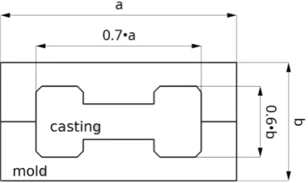
The model described in section II was implemented by authors hereof in C++ language with the use of TalyFEM finite element routines library [18] and PETSc, as a provider of linear algebra algorithms and data structures [19]. The results of calculations taking into account convection are shown for the domain presented in Fig. 1. The boundary con-ditions utilized the following parameters: Newton boundary condition with the environment temperature equal to 300K, the heat exchange coefficient was equal to 10 W/(mK)

Fig. 1: View of the cast and mold with parameterized dimensions.

1000 W/(mK) for heat transfer through a separation layer between the mold and cast.

A summary of the material properties can be found below in Table I (for casting) and Table II (for mold). That properties correspond on a binary alloy Al-2%Cu.

TABLE I: Material properties for casting

Quantity name Unit Value

Densityρs kg/m3 2824

Densityρl kg/m3 ₂₄₉₈

Specific heatcs J/(kg K) 1077

Specific heatcl J/(kg K) 1275

Thermal conductivityλs W/(m K) 262 Thermal conductivityλl W/(m K) 104

Solidus temperatureTs K 853

Liquidus temperatureTl K 926

Solidification temperature K 933

of pure componentTM

Eutectic temperatureTE K 821

Heat of solidificationL J/kg 390000

Solute partition coefficientk – 0.125

Viscosityµ kg/(m s) 0.004

Expansion coefficientβ 1/K 0.0001

Secondary dendrite arm spacingK0 m 1.4·10−11

TABLE II: Material properties for mold

Quantity name Unit Value

Densityρ kg/m3 ₇₅₀₀

Specific heatc J/(kg K) 620 Thermal conductivityλ W/(m K) 40

The computational domain comprised of64180nodes and

125972 triangle finite elements. Time step used in time integration was equal to 0.025s, and time integration used a value of Θ equal to 1 (Euler Backward). Total run time for our simulation was 120s. The results of the computer simulation are presented only for the first 15s, 30s 60s after which most samples showed no significant convection. The results for the four instances are presented. All simulations use linear triangular finite elements. Dimensions of each domain are parametrized according to Figure 1. The base case has size ofa= 1.0mandb= 0.5mand is treated as 100%. Other samples have 75%, 50%, and 25% base lengths. Those four cases allow assessing the importance of convection in solidification.

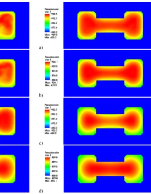
The first series of results present temperature maps for four size of the cast and mold after 15s (Fig. 2), after

30s (Fig. 3), and after 60s (Fig. 4) the time duration of simulations. The more casting size, the more visible is the effect of convection observed as a fluctuation of temperatures during the solidification process. The effect of convection is well visible at the beginning of simulations. With increasing time, the effects of convection are less evident. In each case, according to prediction, the symmetry of results is easily observable.

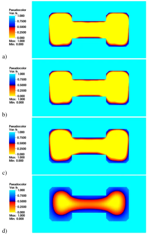
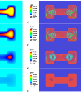
Corresponding solid fraction and velocity maps are pre-sented in Fig. 5, 6, 7, and in Fig. 8, 9, 10, respectively. The liquid phase movement influence on course of solidification process. The bigger size of the cast the more effect of the convection, consequently the slower heat emmision and the slower solidifying.

a)

b)

c)

d)

Fig. 2: Temperature distribution after 15 seconds for a) 100%, b) 75%, c) 50%, and d) 25% dimensions of considered domain.

IV. SUMMARY

a)

b)

c)

d)

Fig. 3: Temperature distribution after 30 seconds for a) 100%, b) 75%, c) 50%, and d) 25% dimensions of considered domain.

make them i) fast, ii) cheap (simulations on workstations), iii) flexible (general-purpose solver), iv) accurate (adaptive error control) [20]. The authors software, which is still in development, satisfies all of these conditions. Future work plans include an experimental comparison of results as the presented model has so far been checked only against benchmark problems.

REFERENCES

[1] Z. Qian, Y. Wang, W. Huai, and Y. Lee, “Numerical simulation of water flow in an axial flow pump with adjustable guide vanes,”Journal Of Mechanical Science And Technology, vol. 24, no. 4, pp. 971–976, 2010.

[2] H. Suito, T. Ueda, and D. Sze, “Numerical simulation of blood flow in the thoracic aorta using a centerline-fitted finite difference approach,”

Japan Journal Of Industrial And Applied Mathematics, vol. 30, no. 3, SI, pp. 701–710, 2013, 4th China-Japan-Korea Conference on Numerical Mathematics, Otsu, JAPAN, AUG 25-28, 2012.

[3] H. Suito and H. Kawarada, “Numerical simulation of spilled oil by fictitious domain method,”Japan Journal Of Industrial And Applied Mathematics, vol. 21, no. 2, pp. 219–236, JUN 2004.

[4] E. Majchrzak and B. Mochnacki, “Application of the shape sensi-tivity analysis in numerical modelling of solidification process,” in

THERMEC 2006, ser. Materials Science Forum, vol. 539. Trans Tech Publications, 2 2007, pp. 2524–2529.

[5] T. Skrzypczak, E. Wgrzyn-Skrzypczak, and L. Sowa, “Numerical modeling of solidification process taking into account the effect of

a)

b)

c)

d)

Fig. 4: Temperature distribution after 60 seconds for a) 100%, b) 75%, c) 50%, and d) 25% dimensions of considered domain.

air gap,”Applied Mathematics and Computation, vol. 321, pp. 768– 779, 2018.

[6] A. Bokota and S. Iskierka, “Finite element method for solving diffusion-convection problems in the presence of a moving heat point source,”Finite Elements in Analysis and Design, vol. 17, no. 2, pp. 89–99, 1994.

[7] T. Skrzypczak, E. Wegrzyn-Skrzypczak, and J. Winczek, “Effect of natural convection on directional solidification of pure metal,”Archives of Metallurgy and Materials, vol. 60, no. 2, pp. 835–841, 2015. [8] D. Stefanescu, Science and Engineering of Casting Solidification.

Springer US, 2009.

[9] W. Feng, Q. Xu, and B. Liu, “Microstructure simulation of aluminum alloy using parallel computing technique,”ISIJ International, vol. 42, no. 7, pp. 702–707, 2002.

[10] E. Gawronska and N. Sczygiol, “Application of mixed time partition-ing methods to raise the efficiency of solidification modelpartition-ing,” in12th Internaitonal Symposium on Symbolic and Numeric Algorithms for Scientific Computing (SYNASC 2010), T. Ida, V. Negru, T. Jebelean, D. Petcu, S. Watt, and D. Zaharie, Eds. Johannes Kepler Univ Linz, Res Inst Symbol Computat; Res Inst e-Austria, 2011, pp. 99–103, 12th International Symposium on Symbolic and Numeric Algorithms for Scientific Computing (SYNASC), W Univ Timisoara, Timisoara, ROMANIA, SEP 23-26, 2010.

[11] E. Gawroska, “A sequential approach to numerical simulations of solidification with domain and time decomposition,”Applied Sciences, vol. 9, p. 1972, 05 2019.

[12] H. Fu, H. Guo, J. Hou, and J. Zhao, “A stabilized mixed finite element method for steady and unsteady reaction-diffusion equations,”

Computer Methods in Applied Mechanics and Engineering, vol. 304, pp. 102–117, 2016.

a)

b)

c)

d)

Fig. 5: Solid fraction distribution after 15 seconds for a) 100%, b) 75%, c) 50%, and d) 25% dimensions of considered domain.

ser. Referex Engineering. Butterworth-Heinemann, 2000.

[14] R. Dyja, E. Gawroska, and A. Grosser, “Numerical problems related to solving the navier-stokes equations in connection with the heat transfer with the use of fem,”Procedia Engineering, vol. 177, pp. 78–85, 12 2017.

[15] F. Brezzi, “On the existence, uniqueness and approximation of saddle-point problems arising from lagrangian multipliers,”ESAIM: Mathe-matical Modelling and Numerical Analysis - Modelisation Mathema-tique et Analyse Numerique, vol. 8, no. R2, pp. 129–151, 1974. [16] A. N. Brooks and T. J. R. Hughes, “Streamline upwind/petrov-galerkin

formulations for convection dominated flows with particular emphasis on the incompressible navier-stokes equations,”Computer Methods in Applied Mechanics and Engineering, pp. 199–259, Sep. 1990. [17] N. Zabaras and D. Samanta, “A stabilized volumeaveraging finite

element method for flow in porous media and binary alloy solidi-fication processes,”International Journal for Numerical Methods in Engineering, vol. 60, pp. 1103–1138, 2004.

[18] H. K. Kodali and B. Ganapathysubramanian, “A computational frame-work to investigate charge transport in heterogeneous organic pho-tovoltaic devices,” Computer Methods In Applied Mechanics And Engineering, vol. 247, pp. 113–129, 2012.

[19] S. Balay, W. D. Gropp, L. C. McInnes, and B. F. Smith, Efficient Management of Parallelism in Object-Oriented Numerical Software Libraries. Boston, MA: Birkh¨auser Boston, 1997, pp. 163–202. [20] G. P. Galdi, J. G. Heywood, and R. Rannacher,Fundamental directions

in mathematical fluid mechanics. Birkh¨auser Boston, 1997, pp. viii, 293 pages. [Online]. Available: http://olin.tind.io/record/123789

a)

b)

c)

d)

a)

b)

c)

d)

Fig. 7: Solid fraction distribution after 60 seconds for a) 100%, b) 75%, c) 50%, and d) 25% dimensions of considered domain.

a)

b)

c)

d)

a)

b)

c)

d)

Fig. 9: Velocity vectors distribution after 30 seconds for a) 100%, b) 75%, c) 50%, and d) 25% dimensions of considered domain.

a)

b)

c)

d)