Abstract— The diffusion equations with nonlocal boundary conditions arise in the mathematical modeling of many physical phenomena. In this paper, we present Padé schemes for the numerical solution of two-dimensional (both homogeneous and inhomogeneous) diffusion equations subject to nonlocal boundary conditions. These numerical schemes are based on (1, 2)Padé and (0,3) Padé approximations to the matrix exponentials arising from the method of lines semidiscretization approach. Numerical solutions for two model problems with known theoretical solutions are obtained. The numerical results prove the accuracy of these schemes.
Index Terms— Diffusion Equations, Nonlocal boundary conditions, Padé schemes, Parabolic Problems.
I. INTRODUCTION
The study of mathematical models for many important applications such as chemical diffusion, heat conduction processes, population dynamics, thermoelasticity, medical science, electrochemistry and control theory give rise the two-dimensional parabolic partial differential equation with nonlocal boundary conditions [1 – 13, 20]. The two-dimensional parabolic partial differential equations with nonlocal boundary conditions and Dirichlet boundary conditions have been studied in many papers [1, 11, 16]. In this paper we will develop two third order new schemes for the numerical solution of two-dimensional diffusion problem with nonlocal boundary conditions. We will use the method of lines semidiscretization approach to transform the model partial differential equation (PDE) into a system of first order, linear, ordinary differential equations (ODEs). The solution of this system of ODEs satisfies a certain recurrence relation involving matrix exponential terms. The approximation of matrix exponential by (1, 2)Padé and (0, 3) – Padé yields the new Padé schemes. We will use the partial fraction decomposition techniques for (1,2) – Padé and (0, 3) – Padé approximants [19] to construct the new efficient numerical schemes.
Manuscript received August 18, 2009.
Mohammad Siddique is Associate Professor of Mathematics at the Department of Mathematics and Computer Science at Fayetteville State University, Fayetteville, NC 28301 USA. (phone: 910-672-2436, fax:
II. NUMERICAL PRELIMINARIES
We consider the diffusion equation in two space variables, that is given by
; 0 , 1, 0
t
u u x y t (2.1) Initial conditions are assumed to be of the form
( , , 0) ( , ), ( , ) ,
u x y f x y x y while the Dirichlet time-dependent boundary conditions are
0 1 0 1
(0, , ) ( , ), 0 , 0 1,
(1, , ) ( , ), 0 , 0 1,
( , 0, ) ( ) ( ), 0 , 0 1,
( ,1, ) ( , ), 0 , 0 1,
u y t y t t T y
u y t y t t T y
u x t x t t T x
u x t x t t T x
(2.2)
with f, o, 1, oand 1 known functions.
The function( )t is to be determined. Nonlocal boundary condition is
1 1
0 0
( , , ) ( ), ( , ) ,
u x y t dxdy t x y
(2.3)where is known function.
We divide both intervals 0 x Land 0 y L into N1 equal subintervals with space mesh
1 L h
N
, xi ih , j
y jhand the timet is discretized in steps of length
k
.
At each time step t tn nk n, 0,1, 2, and we will have a square mesh with N2 points within the square and2
N equally spaced points on each side of the boundary. To approximate the solution u x y t( , , )of (4.1) at each point ( ,x y ti j, )l where i j, 1, 2, ,N and l0,1, 2, . Replacing the spatial derivatives in (4.1) by their second order central difference approximation leads to a system of N2first
order, linear, ordinary differential equations of the form
( ) , 0, ( , , 0) ( , )
dv
Av t t v x y f x y
dt (2.4)
where A is a matrix f order N2and can be split into block
diagonal matrices A1 and A2 given by
1 [ i j]
A a , i j 1, 2,3, , .N
where
* 1
0 i j
A if i j a
if i j
* 1
A is the tridiagonal matrix of order N given by
Numerical Computation of Two-dimensional
Diffusion Equation with Nonlocal Boundary
Conditions
* 1 [ m n]
A a , i j 1, 2,3, , .N
where 2
1 1 1
0 m n
if m n
a if m n or m n
otherwise and 2 2 1 [ l k]
A a
h
, l k 1, 2,3, , .N where
2
1 1
l k
I if l k a
I if l k or l k
and I is the identity matrix of order N.
Solving the system (2.4) subject to the initial condition ( , , 0) ( , )
v x y f x y yields [21],
1 ( ) 0
( ) t A. et s A. ( )
v t e f
s ds, t0 and agrees with( )
( ) . ( ) e . ( )
t k
k A t k s A
t
v t k e v t s ds
,t0, , 2 ,k k (2.5)Approximating the quadrature in (2.5) by the trapezoidal rule yields
[ ( ) ( )]
2
( ) k A. ( ) k kA
t k e t
v tk e v t , t0, , 2 ,k k (2.6) and may takes the form as
1
[
( )]
2 ( 1)k A
n n n n
k
t t
v
e
v
(2.7)III. NUMERICAL SCHEMES
For nm, the approximation of the matrix exponential ekA
by the ( , )n m Padé, denoted byRn m, (kA) yields Lo – stable
Padé numerical schemes (see for details G. D Smith [18]). The approximation of the matrix exponential
e
kA by the(1, 2) Padé, denoted by R1, 2(kA) yields a third order numerical scheme
12 2
1 1
1 2 1
3 3 6 [ ( )] 2 ( )
n n n n
k
v I kA I kA k A v t t
.
(3.1) The approximation of the matrix exponential ekA by the
(0,3)Padé`, denoted byR0, 3(kA) yields the third order scheme
1
2 2 3 3
1 1
1 1
2 6 2
n n n n
k
v
I
kA
k A
k A
v
(3.2) The both schemes involve higher powers of the tridiagonal matrix A bring illconditioning into picture, which may cause computational difficulties and make the scheme computationally less efficient.
To avoid illconditioning, we will use the partial fraction decomposition techniques introduced by Khaliq et al [19] to (3.1) and (3.2), Following Wade et. al. [14], we obtain new numerical schemes for
(1, 2)
Padé and(0,3)
Padé as follows:(1,2) – Padé numerical scheme
1
1 1
2
2 Re (
)
n n n n
k
v
w kA cI
v
. (3.3) where w 1 3.535533905932738i,c 2 1.414213562373095i. (0, 3) – Padé numerical scheme
1 1
1 1 1 2 2 1
2
( ) 2 Re ( ) ( )
( )
n n n
n
k
v w kA c I w kA c I v t
t (3.4) where 1
c 1.596071637983321523112854143997
2 0.70196418100833923844359729280014 1.8073394944520218535764598429640 c i 1
w 1.4756865177957207165190465751319
2 0.7378432588978603582595232875659 0.3650178408010284724444376297915 w i
Extension to Inhomogeneous Problem
By adding a forcing function f x y t( , , ) on right hand side of (2.1), we will have inhomogeneous problem. Following [15], the (1, 2)Padé and (0,3)Padé numerical schemes for inhomogeneous problem are as follows:
(1, 2) – Padé Scheme (Inhomogeneous case)
1 1
2
2 ( )
n n n n
k
v
R y v
(3.5) where
kA c I y 1
w v1 nkw f ( t11 n 1k ) kw f ( t 12 n 2k )and
1
c 2.+1.41421356237309504880168872421i
1
w =-1.-3.53553390593273762200422181052i
11 w =-.18301270189221932338186158538 -1.3194792168823420489501653808i 12 w =0.68301270189221932338186158538 -0.094734345490752999851523343427i 1 3 3 6
and 2 3 3
6
.
(0, 3) – Padé Scheme (Inhomogeneous case)
1 1 2
12
[ 2 ( )]
n n n n
k
v y R y v (3.6) where
kA c I y 1
1w v1 nkw f ( t11 n 1k ) kw f ( t 12 n 2k ) and
kA c I y 2
2w v2 nkw f ( t21 n 1k ) kw f ( t 22 n 2k )1
c 1.596071637983321523112854143997
2 c 0.70196418100833923844359729280014 1.8073394944520218535764598429640i 1
w 1.4756865177957207165190465751319
2
w 0.73784325889786035825952328756592 0.36501784080102847244443762979145i
11 21 12
22
w 0.25964745169791, w 0.66492666056455, w 0.3128364277412 0.472314917248i w 0.3505493716099 0.494190545719i
1
3 3
6
and 2 3 3
6
.
The presence of an integral term in a boundary condition immensely complicates the application of standard numerical techniques. The accuracy of the quadrature must be compatible with the discretization of the differential equation. Cannon et. al. [11] used second order composite trapezoidal rule, whereas Dehghan, M. [2] used fourth order Simpson’s third rule for their fourth order scheme. Noye et. al. [22] used Simpson closed rule and Twizell et. al. [16] used trapezoidal rule to approximate the nonlocal boundary condition (2.3). Following Twizell et. al. [16], we have used Trapezoidal rule to handle the nonlocal boundary condition.
IV. NUMERICAL RESULTS
In this section we demonstrate the performance of (1, 2) – Padé and (0, 3) – Padé. Following [3, 10, 15], we took
1 , 20
h 1
2400
k such that p was kept constant i.e.
2
1 6 k p
h
. We consider three test problems taken from the literature. The exact solutions are known for these problems and are used to test the accuracy of these numerical schemes. The absolute relative errors between the exact and numerical solutions are shown in the tables and the graphs of numerical and exact solutions are also shown.
A. Problem 1. (Twizell et al. [16] , Ishak [17], Siddique [23,24])
We consider the two-dimensional diffusion equation
2 2
2 2 ; 0 , 1, 0
u u u
x y t
t x y
(4.1)
in which uu x y t( , , ), with Dirichlet time-dependent boundary conditions on the boundary
of the squaredefined by the lines x0, y0, x1, y1, given by
( 2 ) (1 2 )
( 2 ) (1 2 )
(0, , ) , 0 , 0 1,
(1, , ) , 0 , 0 1,
( , 0, ) , 0 , 0 1,
( ,1, ) , 0 , 0 1,
y t
y t x t
x t
u y t e t T y
u y t e t T y
u x t e t T x
u x t e t T x
(4.2)
and nonlocal boundary condition
1 1
2 20 0
( , , ) 1 t
u x y t dxdy e e
(4.3)with initial conditions u x y( , , 0)e(x y ). (4.4) Theoretical solution is give by u x y t( , , )e(x y 2 )t . (4.5)
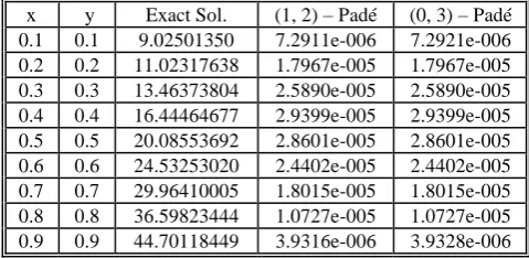
Here the PDE (4.1) subject to (4.2), (4.3) and (4.4) is solved numerically using (1, 2)–Padé and (0, 3)–Padé and schemes. The numerical results for (1, 2)–Padé and (0, 3)–Padé schemes are computed. Following [11, 16, 22], the discretization parameters
h
andk
are given the valuesh
1 ,k
1 . The absolute relative errors for theproblems are tabulated in Table 1 which shows that these schemes gave accurate results. The numerical solutions of (1, 2)–Padé, (0, 3)–Padé and theoretical solution are graphically
[image:3.595.306.546.137.254.2]shown in Figure 1, Figure 2 and Figure 3 respectively. Table 1. Comparing Absolute Relative Error 1 , 1
20 2400
h k
x y Exact Sol. (1, 2) – Padé (0, 3) – Padé 0.1 0.1 9.02501350 7.2911e-006 7.2921e-006 0.2 0.2 11.02317638 1.7967e-005 1.7967e-005 0.3 0.3 13.46373804 2.5890e-005 2.5890e-005 0.4 0.4 16.44464677 2.9399e-005 2.9399e-005 0.5 0.5 20.08553692 2.8601e-005 2.8601e-005 0.6 0.6 24.53253020 2.4402e-005 2.4402e-005 0.7 0.7 29.96410005 1.8015e-005 1.8015e-005 0.8 0.8 36.59823444 1.0727e-005 1.0727e-005 0.9 0.9 44.70118449 3.9316e-006 3.9328e-006 Twizell et. al. [16] have introduced a parallel algorithm based on (1, 2) – Padé approximation to the matrix exponential. The parallel algorithm is implemented on problem 1
for 1 , 1
20 2400
[image:3.595.47.294.440.685.2]h k . The following table is presented in [16].
Table 2. Comparing Absolute Relative Error 1 , 1
20 2400
h k
x y Exact Sol. (1, 2) – Padé Parallel Alg
[image:3.595.321.529.561.694.2](1.5) FTCS 0.1 0.1 9.02501350 3.3993 e-004 3.4000e-003 0.2 0.2 11.02317638 3.2676 e-004 2.2000e-004 0.3 0.3 13.46373804 2.6002 e-004 4.2000e-004 0.4 0.4 16.44464677 1.8408 e-004 1.5000e-004 0.5 0.5 20.08553692 1.1595 e-004 3.2000e-004 0.6 0.6 24.53253020 6.3782 e-005 4.2000e-004 0.7 0.7 29.96410005 2.9338 e-005 4.4000e-004 0.8 0.8 36.59823444 5.1982 e-006 3.5000e-004 0.9 0.9 44.70118449 3.3960 e-006 1.6000e-004
Figure 1. Graph of (0, 3) – Padé numerical scheme
Figure 2. Graph of (1, 2) – Padé numerical scheme
Figure 3. Graph of theoretical solution
B. Problem 2. (Ishak [17], Siddique [23, 24])
We consider the diffusion equation in two space variables, that is given by
2 2
2 2; 0 , 1, 0
u u u
x y t
t x y
(4.6)
subject to the initial condition
( , , 0) (1 ) x, 0 1, 0 1
u x y y e x y (4.7)
And the boundary conditions
1
(0, , ) (1 ) , 0 1, 0 1,
(1, , ) (1 ) , 0 1, 0 1,
( , 0, ) , 0 1, 0 1,
( ,1, ) 0, 0 1, 0 1,
t t x t
u y t y e t y
u y t y e t y
u x t e t x
u x t t x
[image:4.595.330.523.169.295.2](4.8)
Table 3. Comparing Absolute Relative Errors 1 , 1
20 2400
h k
x y Exact Sol. (1, 2) –Padé (0, 3) –Padé 0.1 0.1 2.703749421552 2.5200e-006 2.5203e-006 0.2 0.2 2.656093538189 6.5980e-006 6.5980e-006 0.3 0.3 2.568507667333 1.0448e-005 1.0448e-005 0.4 0.4 2.433119980107 1.3310e-005 1.3310e-005 0.5 0.5 2.240844535169 1.4786e-005 1.4786e-005 0.6 0.6 1.981212969758 1.4698e-005 1.4698e-005 0.7 0.7 1.642184217518 1.3035e-005 1.3035e-005 0.8 0.8 1.209929492883 9.9070e-006 9.9070e-006 0.9 0.9 0.668589444228 5.4944e-006 5.4946e-006
and nonlocal boundary condition
1 (1 )
0 0 ( , , ) 2(11 4 ) , 0 1, 0 1.
x x
t
u x y t dxdy e e x y
(4.9) [image:4.595.71.260.252.381.2]The exact solution is given by u x y t( , , ) (1 y e) x t (4.10)
Figure 4. Graph of (0, 3) – Padé numerical scheme
Figure 5. Graph of (1, 2) – Padé numerical scheme
[image:4.595.330.518.358.477.2] [image:4.595.323.519.528.649.2]C. Problem 3. (Siddique [23, 24]) Consider the
two-dimensional nonhomogeneous diffusion problem
2 2
2 2
2 2 ( 4) , 0, 0 , 1.
t
u u u
e x y t x y
t x y
,
(4.11) The problem has nonsmooth data with the initial condition
2 2
(0, , ) 1
u x y x y (4.12) and the boundary conditions
2
2
2
2
(0, , ) 1 , 0 1, 0 1,
(1, , ) 1 (1 ) , 0 1, 0 1,
( , 0, ) 1 , 0 1, 0 1,
( ,1, ) 1 (1 ) , 0 1, 0 1,
t t t
t
u y t y e t y
u y t y e t y
u x t x e t x
u x t x e t x
(4.13)
and nonlocal boundary condition
1 1
0 0
2 3
( , , ) 1 t, 0 1, 0 1
u x y t dxdy e x y
(4.14) The exact solution is u t x y( , , ) 1 et(x2y2) (4.15)
[image:5.595.306.539.75.377.2]
Figure 7.Graph of (0, 3) – Padé numerical scheme
Figure 8. Graph of (1, 2) – Padé numerical scheme
Table 4. Comparing Absolute Relative Errors 1 , 1
20 2400
h k
x y Exact Sol. (1, 2) – Padé (0, 3) – Padé 0.1 0.1 1.00735759 1.4024e-012 3.3129e-012 0.2 0.2 1.02943036 1.4766e-012 4.3694e-012 0.3 0.3 1.06621830 1.4533e-012 4.2808e-012 0.4 0.4 1.11772142 1.4024e-012 4.1402e-012 0.5 0.5 1.18393972 1.3285e-012 3.9455e-012 0.6 0.6 1.26487320 1.2357e-012 3.6930e-012 0.7 0.7 1.36052185 1.1249e-012 3.3877e-012 0.8 0.8 1.47088568 9.9720e-013 2.8451e-012 0.9 0.9 1.59596469 1.2458e-011 1.7570e-010
Figure 9. Graph of Theoretical solution
The absolute relative errors for problem 2 and 3 are tabulated in Table 3 and 4, which shows that (1, 2) – Padé and (0, 3) – Padé give superior results for problem 3, which is inhomogeneous diffusion equation with nonlocal boundary conditions.
V. CONCLUSION
In this work, we employed new Padé numerical scheme for the solution of two dimensional diffusion equations with nonlocal boundary conditions on four boundaries. To verify the accuracy of these schemes for parabolic problems with nonlocal boundary conditions, numerical solution, exact solution and the absolute relative errors are computed. The numerical results show that these Padé schemes are efficient and provide very accurate results.
REFERENCES
[1] Dehghan, M., Implicit locally one-dimensional methods for two-dimensional diffusion with a nonlocal boundary condition, Math. And Computers in simulation 49 (1999), 331 – 349. [2] Dehghan, M.., A New ADI Technique for the Two Dimensional
Parabolic Equation With an Integral Condition, Int. J. Comp.& Math. With Applications.,43, (1477-1488), 2002.
[3] Cannon, J. R. and van der Hoek, J., Diffusion Subject to the Specification of Mass, J. Math. Anal. Appl., 115, pp. 517-529, 1986.
[4] Cannon, J. R., Y. Lin and S. Wang, ―An Implicit Finite Difference Scheme for the Diffusion Equation Subject to Mass Specification‖, Int. J. Eng. Sci. 28 (1990), 573 – 578.
[image:5.595.70.259.505.634.2][6] Day, W. A., A Decreasing Property of Solutions of a Parabolic Equation with Applications in Thermoelasticity And Other Theories, Quart. Appl. Math., 41, pp. 475 – 486, 1983. [7] Day, W. A., Existence of a Property of Solutions of the Heat
Equation to Linear Thermoelasticity And Other Theories, Quart. Appl. Math., 40, pp. 319 –330, 1982.
[8] Evans, D. J. and Abdullah, A. R., A New Explicit Method For the
Solution of
2 2
2 2
u u u
t x y
. Intern. J. Computer Math., 14, pp. 325-353, 1983.
[9] Wang, S. A numerical method for the heat conduction subject to moving boundary energy specification, Numerical Heat Transfer 130, 35 – 38, 1990.
[10] Wang, S. and Lin, Y., A numerical method for the diffusion equation with nonlocal boundary specifications, Intern. J. Engng. Sci. – 28, 543 – 546, 1991.
[11] Cannon, J. R., Lin, Y. and Matheson A. L, (1993). The solution of the diffusion equation in two-space variables subject to the specification of mass. Applied Analysis, 50(1).
[12] Noye, B. J. and Hayman, K. J., Explicit Two-Level Finite Difference Methods for the Two Dimensional Diffusion Equation, Intern. J. Computer Math., 42, pp. 223-236, 1992. [13] Wang, S. and Lin, Y., A Finite Difference Solution to An Inverse
Problem Determining a Controlling Function in a Parabolic Partial Differential Equation, Inverse Problems, 5, pp. 631-640, 1989.
[14] B. A. Wade, A.Q.M. Khaliq, M. Siddique and M. Yousuf, "Smoothing with Positivity-Preserving Padé Schemes for Parabolic Problems with Nonsmoth Data‖, Numerical Methods for Partial Differential Equations (NMPDE), Wiley Interscience, V. 21, No. 3, 2005, pp. 553--573, DOI 10.1002/num. 20039. [15] B. A. Wade, A.Q.M. Khaliq, M. Yousuf and J. Vigo–Aguiar ―
High Order Smoothing Schemes for Inhomogeneous Parabolic Problems with Applications to Nonsmooth Payoff in Option Pricing" Numerical Methods for Partial Differential Equations (NMPDE) V. 23(5), 2007, 1249--1276.
[16] A. B. Gumel, W. T. Ang and E. H. Twizell, ―Efficient Parallel Algorithm for the Two Dimensional Diffusion Equation Subject to Specification of Mass‖, Intern. J. Computer Math, Vol. 64, p. 153 – 163 (1997).
[17] Ishak Hashim, ―Comparing Numerical Methods for the Solutions of Two-Dimensional Diffusion with an Integral Condition‖, Applied Mathematics and Computation 181 (2006) 880 – 885. [18] G. D. Smith, ―Numerical Solution of Partial Differential
Equations Finite Difference Methods ‖, Third Edition, Oxford University Press, New York (1985).
[19] A. Q. M. Khaliq, E. H. Twizell and D. A. Voss, ― On Parallel Algorithms for Semidiscretized Parabolic Partial Differential Equations Based on Subdiagonal Padé Approximations ‖, (NMPDE), Wiley Interscience, 9, 107 – 116 (1993).
[20] P. Marcati, Some considerations on the mathematical approach to nonlinear age dependent population dynamics, Computers Math. Applic. 9 (3) 361 – 370 (1983).
[21] Y. Lin and S. Wang, ―A Numerical Method for the Diffusion Equation with nonlocal boundary conditions‖, Int. J. Eng. Sci. 28 (1990), 543 – 546.
[22] Noye, B. J., Dehghan, M., and van der Hoek, J., Explicit Finite Difference Methods for the Two Dimensional Diffusion Equation With a Nonlocal Boundary Condition, Int. J. Egg. Sci., 32 (11), pp. 1829-1834, 1994.
[23] Mohammad Siddique, ―A Comparison of Third Order
L o Stable Numerical Schemes for the Two-Dimensional Homogeneous Diffusion Problem Subject to Specification of Mass‖, Applied Mathematical Sciences, vol. 4, 2010, no. 13, 611 – 621.
[24] Mohammad Siddique, ―Smoothing of Crank-Nicolson Schemes for the Two-Dimensional Diffusion with an Integral Condition‖, Applied Mathematics and Computation, 214, 2009, 512 – 522.
Dr. Mohammad Siddique is a dedicated, internationally known, research scholar in Applied Mathematics and is an Associate Professor of Mathematics at the Fayetteville State University, Fayetteville, NC, USA. His outstanding contribution in applied mathematics is designing and analyzing a family of higher order convergent numerical schemes based on Padé approximants, involving both finite differences and finite elements for parabolic partial differential equations with applications in science and engineering. His computational activities that are part of the research include experimentation and prototyping with Maple and Matlab plus parallel processing on a Beowulf cluster using Message Passing Interface (MPI) and C. Dr. Siddique’s research work is published in highly reputed journal. Currently he is working on parabolic problems with nonlocal boundary conditions. He has been a reviewer for many International Conferences (CCCT 2008, CSEI 2009, CCCT 2009, IMETI 2009) and International Journal of Computer Mathematics (IJCM) UK. In the past 3 years, he has organized / chaired invited sessions in several International Conferences of high repute: CMMSE 2007, CCCT 2008, CSEI 2009, CCCT 2009, IMETI 2009, ICNAAM 2009. In addition he is a member of AMS, SIAM, International Scientific Committee WASET, IAENG Society of Scientific Computing., and organizing committee ICNAAM 2010.