Multiwave Solutions for the Toda Lattice Equation
by Generalizing Exp-Function Method
Sheng Zhang, Ying-Ying Zhou
Abstract—In this paper, the exp-function method is gener-alized to construct multiwave solutions of a (2+1)-dimensional variable-coefficient Toda lattice equation. As a result, single-wave solution, double-single-wave solution and three-single-wave solution are obtained, from which the uniform formula of N -wave solution is derived. It is shown that the generalized exp-function method can be used for generating multiwave solutions of some other nonlinear differential-difference equations with variable coefficients.
Index Terms—Multiwave solution, Toda lattice equation, exp-function method, nonlinear differential-difference equation.
I. INTRODUCTION
I
T is the work of Fermi, Pasta and Ulam in the 1950s [1] that has attached much attention on exact solu-tions of nonlinear differential-difference equasolu-tions (DDEs), which play a crucial role in modelling many phenomena in different fields like condensed matter physics, biophysics or mechanical engineering. In the numerical simulation of soliton dynamics in high energy physics, some DDEs of-ten arise as approximations of continuum models. Unlike difference equations which are fully discretized, DDEs are semi-discretized with some (or all) of their spacial variables discretized while time is usually kept continuous. Among the existing DDEs, Toda lattice is a simple model for a nonlinear one-dimensional crystal. The equation of motion of such a lattice system is usually given bymd
2
dt2xn=V ′(x
n+1−xn)−V′(xn−xn−1), (1)
where m denotes the mass of each particle,xn =xn(t) is the displacement of the n-th particle from its equilibrium position, V′(r) = dV(r)/dr,V(r)is the interaction poten-tial. The Toda lattice equation (1) describes the motion of a chain of particles with nearest neighbor interaction [2], different versions of which are often used to construct the mathematical model, for example, the Toda lattice model of DNA in the field of biology [3]. One important property of such type of Toda lattice equations is the existence of so-called soliton solutions (stable waves) which spread in time without changing their size or shape and interact with each other in a particle-like way [4]. There is a close relation between the existence of soliton solutions and the integra-bility of equations, the known research results show that all
Manuscript received March 28, 2014; revised August 30, 2014. This work was supported by the Natural Science Foundation of Liaoning Province of China (L2012404), the Liaoning BaiQianWan Talents Program (2013921055), the PhD Start-up Fund of Liaoning Province of China (20141137) and the Natural Science Foundation of China (11371071).
S. Zhang is with the School of Mathematics and Physics, Bohai Uni-versity, Jinzhou 121013 China, to whom any correspondence should be addressed, e-mail: [email protected].
Y.-Y. Zhou is with the School of Mathematics and Physics, Bohai University, Jinzhou 121013 China, e-mail: [email protected].
the integrable systems exist soliton solutions [5]. Multiwave solutions are a kind of interaction solutions, which include not only classical multisoliton solutions (without singular points) but also singular multisoliton solutions. Usually, the interactions of singular solitons may show entirely different evolution characteristics from those of regular ones.
In the past several decades, there has been significant pro-gression in the development of methods for solving nonlinear partial differential equations (PDEs), such as the inverse scattering method [6], Hirota’s bilinear method [7], B¨acklund transformation [8], Painlev´e expansion [9], homogeneous balance method [10], function expansion methods [11], [12], [13], [14], [15], and others [16], [17], [18], [19], [20]. With the development of soliton theory, finding multiwave solu-tions of nonlinear PDEs and DDEs has gradually developed into a significant direction in nonlinear science. Generally speaking, it is hard to generalize one method for nonlinear PDEs to solve DDEs because of the difficulty in searching for iterative relations from indicesnton±1. Recently, the exp-function method [21] has been proposed and applied to many kinds of nonlinear PDEs [22], [23], [24], [25], [26], [27], [28], [29], [30], [31], [32], [33]. In 2008, Marinakis [34] generalized the exp-function method to obtain multisoliton solutions of the famous Korteweg-de Vries (KdV) equation. Later, Marinakis’ work was improved for obtaining the uniform formula of N-soliton solution of a KdV equation with variable coefficients [35]. More recently, Zhang and Zhang [36] generalized the exp-function method to construct multiwave solutions of nonlinear DDEs by devising a rational ans¨atz of multiple exponential functions. More and more studies show that because of its more general ans¨atz with free parameters, the exp-function method can be used to construct multiple types of exact solutions of many nonlinear PDEs and DDEs.
In the present paper, we shall further generalize the exp-function method to construct multiwave solutions of non-linear DDEs with variable coefficients. In order to illustrate the effectiveness and advantages of the generalized method, we would like to consider a (2+1)-dimensional variable-coefficient Toda lattice equation in the form [37]:
∂2u n ∂x∂t =
[
∂un ∂t +α(t)
]
(un−1−2un+un+1), (2)
where un = un(x, t) and α(t) is an arbitrary function of t. Particularly, when α(t) = 1, Eq. (2) becomes the (2+1)-dimensional constant-coefficient Toda lattice equation [38].
The rest of this paper is organized as follows. In Section 2, we generalize the exp-function method to construct multi-wave solutions of nonlinear DDEs with variable coefficients. In Section 3, we apply the generalized method to Eq. (2). In Section 4, some conclusions are given.
IAENG International Journal of Applied Mathematics, 44:4, IJAM_44_4_03
II. METHODOLOGY
In this section, we describe the basic idea of the general-ized exp-function method with a general ans¨atz for construct-ing multiwave solutions of variable-coefficient nonlinear DDEs, say, in three variablesn,xandt:
△(unt, unx, untt, unxt, . . . un−1, un, un+1,· · ·,) = 0, (3)
where △ is a polynomial of un, un±s(s = 1,2,· · ·) and their derivatives, otherwise, a suitable transformation can transform Eq. (3) into such an equation.
The exp-function method generalized in this paper for single-wave solution is based on the assumption that the solutions of Eq. (3) can be expressed as follows:
un =
∑p1 i1=0ai1e
i1ξ1
∑q1 j1=0bj1e
j1ξ1, (4)
un−s=
∑p1 i1=0ai1e
i1(ξ1−sk1)
∑q1 j1=0bj1e
j1(ξ1−sk1), (5)
un+s=
∑p1 i1=0ai1e
i1(ξ1+sk1)
∑q1 j1=0bj1e
j1(ξ1+sk1), (6)
where ξ1 = k1n+c1(x, t) +ω1, c1(x, t) is an unknown
function ofxandt,ai1,bj1andk1are constants to determine later,ω1is an arbitrary constant, the values ofp1andq1can
be determined by balancing the linear term of highest order in Eq. (3) with the highest order nonlinear term.
In order to seekN-wave solutions for any integerN >1, we generalize Eqs. (4)–(6) as follows:
un=
∑p1 i1=0
∑p2 i2=0· · ·
∑pN
iN=0ai1i2···iNe
∑N g=1igξg
∑q1 j1=0
∑q2 j2=0· · ·
∑qN
jN=0bj1j2···jNe
∑N g=1jgξg
, (7)
un−s=
∑p1 i1=0
∑p2 i2=0· · ·
∑pN
iN=0ai1i2···iNe
∑N
g=1ig(ξg−skg)
∑q1 j1=0
∑q2 j2=0· · ·
∑qN
jN=0bj1j2···jNe
∑N
g=1jg(ξg−skg) ,
(8)
un+s=
∑p1 i1=0
∑p2 i2=0· · ·
∑pN
iN=0ai1i2···iNe
∑N
g=1ig(ξg+skg)
∑q1 j1=0
∑q2 j2=0· · ·
∑qN
jN=0bj1j2···jNe
∑N
g=1jg(ξg+skg) ,
(9) whereξg=kgn+cg(x, t) +ωg. When N= 2, Eqs. (7)–(9) give:
un=
∑p1 i1=0
∑p2
i2=0ai1i2e
∑2
g=1igξg
∑q1 j1=0
∑q2
j2=0bj1j2e
∑2
g=1jgξg
, (10)
un−s=
∑p1 i1=0
∑p2
i2=0ai1i2e
∑2
g=1ig(ξg−skg)
∑q1 j1=0
∑q2
j2=0bj1j2e
∑2
g=1jg(ξg−skg)
, (11)
un+s=
∑p1 i1=0
∑p2
i2=0ai1i2e
∑2
g=1ig(ξg+skg)
∑q1 j1=0
∑q2
j2=0bj1j2e
∑2
g=1jg(ξg+skg)
, (12)
which can be used to construct double-wave solution of Eq. (3).
WhenN = 3, Eqs. (7)–(9) give:
un =
∑p1 i1=0
∑p2 i2=0
∑p3
i3=0ai1i2i3e
∑3
g=1igξg
∑q1 j1=0
∑q2 j2=0
∑q3
j3=0bj1j2j3e
∑3
g=1jgξg
, (13)
un−s=
∑p1 i1=0
∑p2 i2=0
∑p3
i3=0ai1i2i3e
∑3
g=1ig(ξg−skg)
∑q1 j1=0
∑q2 j2=0
∑q3
j3=0bj1j2j3e
∑3
g=1jg(ξg−skg) ,
(14)
un+s=
∑p1 i1=0
∑p2 i2=0
∑p3
i3=0ai1i2i3e
∑3
g=1ig(ξg+skg)
∑q1 j1=0
∑q2 j2=0
∑q3
j3=0bj1j2j3e
∑3
g=1jg(ξg+skg) ,
(15) which can be used to obtain three-wave solution of Eq. (3). Substituting Eqs. (10)–(12) into Eq. (3), and using Math-ematica, then equating each coefficient of the same order power of exponential functions to zero yields a set of differ-ential equations. Solving the set of differdiffer-ential equations, we can determine the double-wave solution, and the following three-wave solution by the use of Eqs. (13)–(15), provided they exist. If possible, we may conclude with the uniform formula ofN-wave solution for any integer N≥1.
III. MULTIWAVE SOLUTIONS
In this section, let us apply the generalized exp-function method described in Section 2 to Eq. (2). To seek single-wave solution, we suppose that:
un(x, t) = a1eξ1
1 +b1eξ1
, (16)
un−1(x, t) =
a1eξ1−k1
1 +b1eξ1−k1
, (17)
un+1(x, t) =
a1eξ1+k1
1 +b1eξ1+k1
, (18)
whereξ1=k1n+c1(x, t)+ω1. Obviously, Eqs. (16)–(18) are
embedded in the same form as Eqs. (4)–(6). Substituting Eqs. (16)–(18) into Eq. (2), and usingMathematica, then equating each coefficient of the same order power of exponential functions to zero yields a set of PDEs as follows:
−a1α(t) + 2a1α(t)ek1−a1α(t)e2k1
+a1c1x(x, t)c1t(x, t)ek1+a1c1xt(x, t)ek1 = 0,
−a1b1α(t) + 2a1b1α(t)ek1−a1b1α(t)e2k1−a21c1t(x, t)
+2a2
1c1t(x, t)ek1−a21c1t(x, t)ek1
+a1b1c1x(x, t)c1t(x, t)−a1b1c1x(x, t)c1t(x, t)ek1
+a1b1c1x(x, t)c1t(x, t)e2k1+a1b1c1xt(x, t)
+a1b1c1xt(x, t)ek1+a1b1c1xt(x, t)e2k1= 0,
a1b21α(t)−2a1b21α(t)ek1+a1b21α(t)e2k1+a21b1c1t(x, t)
−2a21b1c1t(x, t)ek1+a21b1c1t(x, t)e2k1
−a1b21c1x(x, t)c1t(x, t) +a1b21c1x(x, t)c1t(x, t)ek1
−a1b21c1x(x, t)c1t(x, t)e2k1+a1b21c1xt(x, t)
+a1b21c1xt(x, t)ek1+a1b21c1xt(x, t)e2k1= 0,
a1b31α(t)−2a1b31α(t)e k1+a
1b31α(t)e 2k1
−a1b31c1x(x, t)c1t(x, t)ek1+a1b31c1xt(x, t)ek1 = 0. Solving the set of PDEs, we have
a1=b1d1, c1(x, t) =d1x+
4sinhk1
2
d1
∫
α(t)dt. (19)
We, therefore, obtain the single-wave solution of Eq. (2):
un=
b1d1eξ1
1 +b1eξ1
= [ln(1 +b1eξ1)]x, (20)
IAENG International Journal of Applied Mathematics, 44:4, IJAM_44_4_03
whereξ1 =k1n+d1x+ 4sinhk1
2 d1
∫
α(t)dt+ω1,b1,d1,k1
andω1 are arbitrary constants.
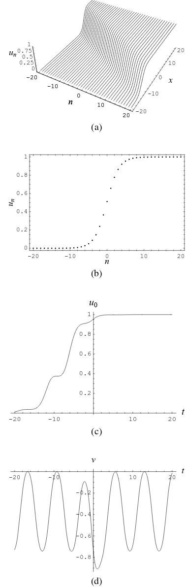
In Fig. 1, the evolution characteristics of a single-kink soliton determined by solution (20) is shown, where we selected k1 = 0.6, b1 = 2, d1 = 1, ω1 = 0, α(t) =
1+secht+sn(t,0.5). Fig. 1(c) shows the asymptotic property of amplitudeu0 atx= 3. Fig. 1(d) shows that the velocity
of un periodically changes with time.
To construct double-wave solution, we suppose that:
un =
a10eξ1+a01eξ2+a11eξ1+ξ2
1 +b1eξ1+b2eξ2+b3eξ1+ξ2
, (21)
un−1=
a10eξ1−k1+a01eξ2−k2+a11eξ1+ξ2−k1−k2
1 +b1eξ1−k1+b2eξ2−k2+b3eξ1+ξ2−k1−k2
, (22)
un+1=
a10eξ1+k1+a01eξ2+k2+a11eξ1+ξ2+k1+k2
1 +b1eξ1+k1+b2eξ2+k2+b3eξ1+ξ2+k1+k2
, (23)
whereξi=kin+ci(x, t) +ωi(i= 1,2). Clearly, Eqs. (21)– (23) possess the same form as Eqs. (10)–(12). Substituting Eqs. (21)–(23) into Eq. (2), and using the similar manipula-tions as illustrated above, we get a set of PDEs. Solving the set of PDEs, we have
a10=b1d1, a01=b2d2, (24)
a11=b1b2(d1+d2)eB12, b3=b1b2eB12, (25)
ci(x, t) =dix+
4sinhki
2
di
∫
α(t)dt (i= 1,2), (26)
eB12 =d
2
1Ω22+d22Ω21−2d1d2Ω1Ω2cosh(k21 −k22)
d2
1Ω22+d22Ω21−2d1d2Ω1Ω2cosh(k21 + k2
2)
, (27)
Ωi= sinh2 ki
2 (i= 1,2). (28) Thus, we obtain the double-wave solution of Eq. (2):
un =
b1d1eξ1+b2d2eξ2+b1b2(d1+d2)eξ1+ξ2+B12
1 +b1eξ1+b2eξ2+b1b2eξ1+ξ2+B12
=[ln(1 +b1eξ1+b2eξ2+b1b2eξ1+ξ2+B12)
]
x,
(29)
where ξi =kin+dix+ 4sinhki2
di
∫
α(t)dt+ωi (i = 1,2), b1,b2,d1,d2,k1,k2,ω1 andω2 are free constants, eB12 is
defined by Eqs. (27) and (28).
In Fig. 2, the evolution characteristics of a double-kink soliton determined by solution (29) is shown, wherek1= 1,
k2= 0.3,b1= 1, b2= 2,d1= 1,d2= 1,ω1= 0,ω2 = 0,
α(t) = 1+secht+sn(t,0.5). Fig. 3 shows a singular double-kink soliton determined by solution (29), all the parameters of which are same as those of Fig. 2 exceptb1=−1. It is
easy to see from Fig. 3 that u0 increases to infinite rapidly
ast→ −5andunhas a jump whenn= 10,x=−8,t= 0. We now construct three-wave solution, for this purpose, we suppose that:
un=
f1,n(ξ1, ξ2, ξ3)
f2
2,n(ξ1, ξ2, ξ3)
, (30)
un−1=
f1,n−1(ξ1, ξ2, ξ3)
f2
2,n−1(ξ1, ξ2, ξ3)
, (31)
un+1=
f1,n+1(ξ1, ξ2, ξ3)
f2
2,n+1(ξ1, ξ2, ξ3)
, (32)
-20 -10
0 10
20
n
-20 -10
0 10
20
x
0 0.25 0.5 0.75 1
un
-20 -10
0 10
20
n
(a)
-20 -10 0 10 20
n 0
0.2 0.4 0.6 0.8 1
un
(b)
-20 -10 10 20
t
0.2 0.4 0.6 0.8 1
u0
(c)
-20 -10 10 20
t
-0.8 -0.6 -0.4 -0.2 v
[image:3.595.328.517.55.651.2](d)
Fig. 1. Evolution plots of single-soliton determined by solution (20): (a)
t= 0; (b)x= 0,t= 0; (c)n= 0,x= 3; (d) velocity curve.
whereξi=kin+ci(x, t) +ωi (i= 1,2,3), and
f1,n(ξ1, ξ2, ξ3) =a100eξ1+a010eξ2+a001eξ3+a110eξ1+ξ2
+a101eξ1+ξ3+a011eξ2+ξ3+a111eξ1+ξ2+ξ3,
f2,n(ξ1, ξ2, ξ3) = 1 +b1eξ1+b2eξ2+b3eξ3+b4eξ1+ξ2
+b5eξ1+ξ3+b6eξ2+ξ3+b7eξ1+ξ2+ξ3,
IAENG International Journal of Applied Mathematics, 44:4, IJAM_44_4_03
-20 -10
0 10
20
n
-20 -10
0 10
20
x
0 0.5 1 1.5 2
un
-20 -10
0 10
20
n
(a)
-20 -10
0
10
n
-10 0
10
t
0 0.5 1 1.5
2
un
-20 -10
0
10
n
(b)
-20 -10 10 20
t
1.2 1.4 1.6 1.8 2
u0
(c)
-30 -20 -10 0 10 20 30
n 0
0.25 0.5 0.75 1 1.25 1.5 1.75
un
[image:4.595.72.525.46.661.2](d)
Fig. 2. Evolution plots of double-solution determined by solution (29): (a)
t= 0; (b)x= 0; (c)n= 0,x= 0; (d)x=−8,t= 0.
f1,n−1(ξ1, ξ2, ξ3) =a100eξ1−k1+a010eξ2−k2+a001eξ3−k3
+a110eξ1+ξ2−k1−k2+a101eξ1+ξ3−k1−k3
+a011eξ2+ξ3−k2−k3+a111eξ1+ξ2+ξ3−k1−k2−k3,
f2,n−1(ξ1, ξ2, ξ3) = 1 +b1eξ1−k1+b2eξ2−k2+b3eξ3−k3
+b4eξ1+ξ2−k1−k2+b5eξ1+ξ3−k1−k3+b6eξ2+ξ3−k2−k3
+b7eξ1+ξ2+ξ3−k1−k2−k3,
-20 -10
0 10
20
n
-20 -10
0 10
20
x
-2 0 2 4
un
-20 -10
0 10
20
n
(a)
-20 -10
0
10
n
-10 0
10
t
-2 0 2 4
un
-20 -10
0
10
n
(b)
-20 -10 10 20
t
-60 -40 -20 20
u0
(c)
-30 -20 -10 0 10 20 30
n 0
2 4 6 8
un
[image:4.595.328.518.50.663.2](d)
Fig. 3. Evolution plots of singular double-soliton determined by solution (29): (a)t= 0; (b)x= 0; (c)n= 0,x= 0; (d)x=−8,t= 0.
f1,n+1(ξ1, ξ2, ξ3) =a100eξ1+k1+a010eξ2+k2+a001eξ3+k3
+a110eξ1+ξ2+k1+k2+a101eξ1+ξ3+k1+k3
+a011eξ2+ξ3+k2+k3+a111eξ1+ξ2+ξ3+k1+k2+k3,
f2,n+1(ξ1, ξ2, ξ3) = 1 +b1eξ1+k1+b2eξ2+k2+b3eξ3+k3
+b4eξ1+ξ2+k1+k2+b5eξ1+ξ3+k1+k3+b6eξ2+ξ3+k2+k3
+b7eξ1+ξ2+ξ3+k1+k2+k3.
IAENG International Journal of Applied Mathematics, 44:4, IJAM_44_4_03
It is easy to see that Eqs. (30)–(32) have the same form as Eqs. (13)–(15). By the similar manipulations mentioned above, we have
a100=b1d1, a010=b2d2, a001=b3d3, (33)
a110=b1b2d1d2eB12, a101=b1b3d1d3eB13, (34)
a011=b2b3d2d3eB23, (35)
a111=b1b2b3(d1+d2+d3)eB12+B13+B23, (36)
b4=b1b2eB12, b5=b1b3eB13, b6=b2b3eB23, (37)
b7=b1b2b3eB12+B13+B23, (38)
ci(x, t) =dix+
4sinhki
2
di
∫
α(t)dt (i= 1,2,3), (39)
eBij =d
2 iΩ
2 j+d
2 jΩ
2
i −2didjΩiΩjcosh(k2i − kj
2)
d2 iΩ
2 j+d
2 jΩ
2
i −2didjΩiΩjcosh(k2i +k2i) , (40)
Ωi= sinh2 ki
2, Ωj = sinh
2kj
2 (1≤i < j≤3). (41) Employing Eqs. (33)–(41), we obtain the three-wave solution of Eq. (2):
un=
[
ln(1 +b1eξ1+b2eξ2+b3eξ3+b1b2eξ1+ξ2+B12
+b1b3eξ1+ξ3+B13+b2b3eξ2+ξ3+B23
+b1b2b3eξ1+ξ2+ξ3+B12+B13+B23)
]
x,
(42)
whereξi=kin+dix+ 4sinhki2
di
∫
α(t)dt+ωi (i= 1,2,3), b1,b2,b3,d1,d2,d3,k1,k2,k3,ω1,ω2 andω3are arbitrary
constants, B12, B13 and B23 are determined by Eqs. (40)
and (41).
In Fig. 4, the evolution characteristics of a three-kink soliton determined by solution (42) is shown, the parameters of which are selected as k1 = 1, k2 = −1, k3 = 0.36,
b1 = 2, b2 = 1, b3 = 3,d1 = 1, d2 = 1, d3 = 2,ω1 = 0,
ω2= 0,ω3= 0,α(t) = 1 + secht+t2.
If we continue to construct the N-wave solution for any N ≥4, the following similar manipulations become rather complicated since equating the coefficients of the exponential functions to zero implies a highly nonlinear system as pointed out in [34]. Fortunately, by analyzing the obtained solutions (20), (29) and (42) we can obtain the uniform formula ofN-wave solution as follows:
un=
[
ln
( ∑
µ=0,1 N
∏
i=1
bµi
i e
∑N i=1µiξi+
∑
1≤i<j≤NµiµjBij
)]
x ,
(43) where the summation ∑µ=0,1 refers to all combinations of eachµi= 0,1fori= 1,2,· · ·, N,ξi=kin+dix+
4sinhki2 di ,
and
eBij =d
2 iΩ
2 j+d
2 jΩ
2
i −2didjΩiΩjcosh(k2i − kj
2)
d2 iΩ
2 j+d
2 jΩ
2
i −2didjΩiΩjcosh(k2i +k2i) , (44)
Ωi= sinh2 ki
2, Ωj = sinh
2kj
2 (i < j;i, j= 1,2,· · ·, N). (45)
Remark 1.Solutions (20), (29) and (42) obtained above have been checked with Mathematicaby putting them back into the original Eq. (2). To the best of our knowledge, solutions (20), (29), (42) and (43) with arbitrary function α(t)have not been reported in literatures.
-20 -10
0 10
20
n
-20 -10
0 10
20
x
0 1 2 3 4
un
-20 -10
0 10
20
n
(a)
-20 -10
0
10
n
-10 0
10
t
0 1 2 3 4
un
-20 -10
0
10
n
(b)
-20 -10 10 20
t
1 2 3 4
u0
(c)
-30 -20 -10 0 10 20 30
n 0
0.5 1 1.5 2 2.5
un
[image:5.595.322.519.46.667.2](d)
Fig. 4. Evolution plots of three-soliton determined by solution (42): (a)
t= 0; (b)x= 0; (c)n= 0,x= 0; (d)x=−6,t= 0.
IV. CONCLUSION
In summary, single-wave solution (20), double-wave so-lution (29) and three-wave soso-lution (42) of the (2+1)-dimensional variable-coefficient Toda lattice equation (2) have been obtained, from which the uniform formula of N-wave solution (43) is derived. This is due to the
general-IAENG International Journal of Applied Mathematics, 44:4, IJAM_44_4_03
ization of the exp-function method presented in this paper. Though these solutions can be constructed by some a future improvement of Hirota’s bilinear method [7], the proposed method with the help of Mathematica for generating solu-tions (20), (29) and (42) is more simple and straightforward. Hirota’s bilinear method has three steps [36], one of which is taking a transformation of new dependent variable(s) to reduce a given DDE to bilinear form(s). However, no general method has been found for such a transformation. Compared to Hirota’s bilinear method, the method of this paper does not follow these steps. Besides, the multiwave solutions constructed by the generalized exp-function method contain free parametersb1,b2,· · ·,bN so that they are more general than the ones(bi = 1, i= 1,2,· · ·, N)obtained by Hirota’s bilinear method. More importantly, these multiwave solutions with free parameters maybe possess new evolution character-istics. For example, when any one parameter is negative, the multiwave solutions can give singular multisoliton solutions like the one (b1 =−1) shown in Fig. 3. In this sense, we
may conclude that the generalized exp-function method with the advantage of simplicity and effectiveness may provide us with a straightforward and applicable mathematical tool for generating multiwave solutions of some variable-coefficient DDEs or testing their existence.
ACKNOWLEDGMENT
The authors would like to express their sincere thanks to anonymous reviewers for the valuable suggestions and comments.
REFERENCES
[1] E. Fermi, J. Pasta, and S. Ulam, Collected Papers of Enrico Fermi. Chicago: Chicago University Press, 1965.
[2] G. Teschl, Jacobi Operators and Completely Integrable Nonlinear Lattices. Rhode Island: American Mathematical Society, 2000. [3] V. Muto, A. C. Scott, and P. L. Christiansen, “Thermally generated
solitons in a Toda lattice model of DNA,”Physics Letters Avol. 136, no. 1-2, pp. 33-36, Mar. 1989.
[4] G. Teschl, “Almost everything you always wanted to know about the Toda equation,”Jahresber Deutsch Math-Vereinvol. 103, no. 4, pp. 149-162, Apr. 2001.
[5] S. Y. Lou and X. Y. Tang, Method of Nonlinear Mathematical Physics. Beijing: Science Press, 2006.
[6] C. S. Gardner, J. M. Greene, M. D. Kruskal, and R. M. Miura, “Method for solving the Korteweg–de Vries equation,”Physical Review Letters
vol. 19, no. 19, pp. 1095-1097, Nov. 1967.
[7] R. Hirota, Exact solution of the Korteweg–de Vries equation for multiple collisions of solitons,Physical Review Lettersvol. 27, no. 18, pp. 1192-1194, Nov. 1971.
[8] M. R. Miurs, B¨acklund Transformation. Berlin: Springer, 1978. [9] J. Weiss, M. Tabor, and G. Carnevale, “The Painlev´e property for
partial differential equations,”Journal of Mathematical Physicsvol. 24, no. 3, pp. 522-526, Mar. 1983.
[10] M. L. Wang, “Exact solutions for a compound KdV–Burgers equation,”
Physics Letters Avol. 213, no. 5-6, pp. 279-287, Apr. 1996. [11] E. G. Fan, “Travelling wave solutions in terms of special functions for
nonlinear coupled evolution systems,”Physics Letters Avol. 300, no. 2-3, pp. 243-249, Jul. 2002.
[12] E. G. Fan and H. H. Dai, “A direct approach with computerized symbolic computation for finding a series of traveling waves to nonlinear equations,” Computer Physics Communications vol. 153, no.1, pp. 17-30, Jun. 2003.
[13] N. N. Shang and B. Zheng, “Exact solutions for three fractional partial differential equations by the (G’/G) method,” IAENG International Journal of Applied Mathematics, vol. 43, no. 3, pp. 114-119, Aug. 2013.
[14] E. Yomba, “The modified extended Fan sub-equation method and its application to the (2+1)-dimensional Broer–Kaup–Kupershmidt equation,”Chaos, Solitons & Fractalsvol. 27, no. 1, pp. 187-196, Jan. 2007.
[15] S. Zhang and T.C. Xia, “A generalized auxiliary equation method and its application to (2+1)-dimensional asymmetric Nizhnik–Novikov– Vesselov equations,”Journal of Physics A: Mathematical and Theo-reticalvol. 40, no. 2, pp. 227-248, Jan. 2007.
[16] W. X. Ma, T. W. Huang, and Y. Zhang, “A multiple exp-function method for nonlinear differential equations and its application,” Phys-ica Scripta, vol. 82, no. 6, 065003(8pp.), Dec. 2010.
[17] A. El-Ajou, Z. Odibat, S. Momani, and A. Alawneh, “Construction of analytical solutions to fractional differential equations using homotopy analysis method,”IAENG International Journal of Applied Mathemat-ics, vol. 40, no. 2, pp. 43-51, May 2010.
[18] Y. Huang, “Explicit multi-soliton solutions for the KdV equation by Darboux transformation,” IAENG International Journal of Applied Mathematics, vol. 43, no. 3, pp. 135-137, Aug. 2013.
[19] C. Q. Dai, Y. Y. Wang, Q. Tian, and J. F. Zhang, “The management and containment of self-similar rogue waves in the inhomogeneous nonlinear Schr¨odinger equation,” Annals of Physicsvol. 327, no. 2, pp. 512-521, Feb. 2012.
[20] C. Q. Dai, X. G. Wang, and G. Q. Zhou, “Stable light-bullet solu-tions in the harmonic and parity-time-symmetric potentials,”Physical Review Avol. 89, no. 1, 013834(7pp.), Jan. 2014.
[21] J. H. He and X. H. Wu, “Exp-function method for nonlinear wave equations,”Chaos, Solitons & Fractals, vol. 30, no. 3, pp. 700-708, Nov. 2006.
[22] J. H. He and M. A. Abdou, “New periodic solutions for nonlinear evolution equations using Exp-function method,” Chaos, Solitons & Fractalsvol. 34, no. 5, pp. 1421-1429, Dec. 2007.
[23] J. H. He and L. N. Zhang, “Generalized solitary solution and compacton-like solution of the Jaulent–Miodek equations using the Exp-function method,”Physics Letters Avol. 372, no. 7, 1044-1047, Feb. 2007.
[24] X. H. Wu and J. H. He, “Solitary solutions, periodic solutions and compacton-like solutions using the Exp-function method,”Computers & Mathematics with Applications vol. 54, no. 7-8, pp. 966-986, Oct. 2007.
[25] S. Zhang, “Application of Exp-function method to a KdV equation with variable coefficients,” Physics Letters Avol. 365, no. 5-6, pp. 448-453, Jun. 2007.
[26] S. D. Zhu, “Exp-function method for the hybrid-lattice system,”
International Journal of Nonlinear Sciences and Numerical Simulation
vol. 8, no. 3, pp. 461-464, Sep. 2007.
[27] A. Boz and A. Bekir, “Application of exp-function method for (3+1)-dimensional nonlinear evolution equations,”Computers & Mathemat-ics with Applications, vol. 56, no. 5, pp. 1451-1456, Sep. 2008. [28] C. Q. Dai and J. L. Chen, “New analytic solutions of stochastic coupled
KdV equations,”Chaos, Solitons & Fracatalsvol. 42, no. 4, pp. 2200-2207, Nov. 2009.
[29] A. Ebaid, “Exact solitary wave solutions for some nonlinear evolution equations via Exp-function method,”Physics Letters Avol. 365, no. 3, pp. 213-219, May 2012.
[30] M. A. Abdou, “Generalized solitonary and periodic solutions for nonlinear partial differential equations by the Exp-function method,”
Nonlinear Dynamicsvol. 52, no. 1-2, pp. 1-9, Apr. 2008.
[31] I. Aslan, “On the application of the Exp-function method to the KP equation forN-soliton solutions,”Applied Mathematics and Compu-tationvol. 219, no. 6, pp. 2825-2828, Nov. 2012.
[32] L. Zhao, D. J. Huang, and S. G. Zhou, “A new algorithm for automatic computation of solitary wave solutions to nonlinear partial differential equations based on the Exp-function method,”Applied Mathematics and Computationvol. 219, no. 4, pp. 1890-1896, Nov. 2012. [33] S. Zhang, “Exp-function method: solitary, periodic and rational wave
solutions of nonlinear evolution equations,”Nonlinear Sciecne Letters Avol. 1, no. 2, pp. 143-146, Jun. 2010.
[34] V. Marinakis, The Exp-function method find n-soliton solutions,
Zeitschrift fur Naturforschung Avol. 63, no. 10-11, pp. 653-656, Oct. 2008.
[35] S. Zhang and H. Q. Zhang, “Exp-function method for N-soliton solutions of nonlinear evolution equations in mathematical physics,”
Physics Letters Avol. 373, no. 30, pp. 2501-2505, Jul. 2009. [36] S. Zhang and H. Q. Zhang, “Exp-function method for N-soliton
solutions of nonlinear differential-difference equations,”Zeitschrift fur Naturforschung Avol. 65, no. 11, pp. 924-934, Nov. 2010.
[37] S. Zhang, Q. A. Zong, Q. Gao, and D. Liu, “A (2+1)-dimensional nonlinear differential-difference equation arising in natotechnology and its exact solutions,”Advanced Science Lettersvol. 10, no. 1, pp. 693-695, May 2012.
[38] S. Zhang and H. Q. Zhang, “Variable-coefficient discrete tanh method and its application to (2+1)-dimensional Toda equation.” Physics Letters Avol. 373, no. 33, pp. 2905-2910, Aug. 2009.