Abstract—In this paper, a numerical method based on Legendre polynomials is proposed for solving the variable order time fractional diffusion equation. We adopt the Coimbra variable order time fractional operator, which can be viewed as a Caputo-type definition. Operational matrix of differentiation is also introduced. Combining this matrix with the properties of Legendre polynomials, we transform the initial problem into a Sylvester equation. Numerical example is provided to demonstrate the validity and applicability of the technique. Moreover, comparing the methodology with the known method shows that our approach is more efficient and more convenient.
Keywords—Variable order; Legendre polynomials; Operational matrix; Sylvester equation; Numerical solution
I. INTRODUCTION
n science and engineering, many dynamical systems can be described by fractional-order equation [1-3]. These dynamical systems generally originates in the fields of electrode-electrolyte [4], dielectric polarization [5], electromagnetic waves [6] and viscoelastic systems [7] etc. Various materials and processes have been found to be described using fractional calculus. Anomalous diffusion has been discussed in various physical fields [8-10]. The features of anomalous diffusion include history dependence, long-range, correlation and heavy tail characteristics. These features can be accommodated well by using fractional calculus. In order to deal with the diffusion processes in which the diffusion behaviors depend on time evolution, space variation, the variable-order diffusion models were proposed. The concept of variable order operator was first introduced by Samko[11-12] in 1993 and received much attention in the fields of viscoelasticity, viscoelastic deformation, viscous fluid. Nowadays, it has been employed as a powerful tool in complex anomalous diffusion modeling.
Up until now, to the best of the authors knowledge, the main approach for solving the variable order time fractional diffusion equation is finite difference method. Lin et al. [13] applied an explicit finite difference method to investigate stability and convergence of approximation for the variable
Manuscript received October 10, 2016; revised May 16, 2017.
Nanyu Chen is with the School of Aeronautic Science and Engineering, Beihang University, Beijing, P.R.China.
Jun Huang (Corresponding author) is with the School of Aeronautic Science and Engineering, Beihang University, Beijing, P.R.China (e-mail: [email protected]).
Yacong Wu and Qian Xiao are with the School of Aeronautic Science and Engineering, Beihang University, Beijing, P.R.China.
order nonlinear fractional diffusion equation. Zhuang et al. [14] proposed explicit and implicit Euler method for the variable order fractional advection-diffusion equation. Chen et al. [15] used two numerical methods to solve the variable order anomalous sub-diffusion equation.
Legendre polynomials play a prominent role in various areas of mathematics. These polynomials have frequently used in both the solution of differential equations and approximation theory [16-17]. Abbasbandy et.al. [18] presented the operational matrix method based on fractional order Legendre polynomials for the time fractional convection diffusion equations. Islam and Hossain [19] used the Bernstein and Legendre polynomials to solve the eighth order boundary value problem.
In this study, we consider the following variable order time fractional diffusion equation:
2 ( , )
2
( , )
( , ) ( , ),
( , ) [0,1] [0,1]
q x t t
u x t
D u x t f x t
x x t
(1)
with initial and boundary conditions
( , 0) ( ), 0 1
u x g x x (2)
(0, ) (1, ) 0, 0 1
u t u t t (3) where 0q x t( , )1, f x t( , ) and g x( ) are the known functions. Dtq x t( , ) denotes the variable order time fractional
derivative defined by Coimbra [20]:
( , ) ( , )
0
( , )
1 ( , )
( , ) ( )
(1 ( , ))
( ( , 0 ) ( , 0 )) (1 ( , ))
t
q x t q x t
t
q x t u x
D u x t t d
q x t
u x u x t
q x t
(4)
For the sake of simplicity, assuming u x( , 0 ) u x( , 0 ) , then the Coimbra definition can be viewed as the following Caputo-type definition:
( , ) ( , )
0
1 ( , )
( , ) ( ) (1 ( , ))
t
q x t q x t
t
u x
D u x t t d
q x t
(5)II. LEGENDRE POLYNOMIALS AND THEIR SOME PROPERTIES
The Legendre basis polynomials of degree n in
[0,1]are defined by [16]
1 1
(2 1)(2 1)
( ) ( ) ( ), 1, 2, ( 1) 1
i i i
i x i
P x P x P x i
i i
(6)
where P x0( )1, P x1( )2x1. The Legendre polynomials of degree i can be also given by
Operational Matrix Method for the Variable
Order Time Fractional Diffusion Equation
Using Legendre Polynomials Approximation
Nanyu Chen, Jun Huang*, Yacong Wu, Qian Xiao
I
IAENG International Journal of Applied Mathematics, 47:3, IJAM_47_3_07
2 0
( )! ( ) ( 1)
( )! ( !) k i i k i k
i k x P x
i k k
(7)Let
T0 , 1 , , n x P x P x P x
Φ (8)
The Legendre polynomials given by Eq.(6) can be expressed in the matrix form
x n
xΦ A (9)
where
2
2 3
1 2
1 0 0
1 ( 1) 2! 0
3!
( 1) ( 1) 0
1!
( 1)! (2 )!
( 1) ( 1) ( 1)
( 1)! !
n n n n n
n n A (10) Obviously
1
n x x
A
(11)
A function u x t( , )L2([0,1] [0,1]) can be expressed in terms of the Legendre basis. In practice, only the first
(n 1) (n 1)term of Legendre polynomials are considered. Hence
0 0
( , ) ( ) ( ) ( ) ( )
n n
T ij n n i j
u x t c P x P t x t
C (12)where
00 01 0
10 11 1
0 1
n
n
n n nn
c c c
c c c
c c c
C , cijare called Legendre
coefficients.
Theorem 1. For any x ti, j[0,1], suppose that the function
( , )
n
u x t x
obtained by using Legendre polynomials are the
approximation of u x t( , )
x
, q x t( , )i j , and u x t( , )has
bounded mixed fractional partial derivative
4 2 2
( , ) ˆ
u x t M x t
, then we have
ˆ ( , )
( , ) ( 0.5)
8 ( 0.5)
n E u x t
u x t M n
n x x
where
1/2 1 1 2
1 1
( ) E ( )
u x,t u x,t dxdt
and1 1 1 1
2 1 2 1 ( , )
( ) ( )
2 2
ij i j
i j u x t
u P x P t dxdt
x
.Proof. The property of the
P xi( )
on [ 1,1] implies that1 1
2
, ;
( ) ( ) 2 1 0,
i j
i j P x P x dx i
i j
, then 2 2 1 1 1 1 2 1 1 1 1 1 11 1 2 2 2
1 1
1 1
1
2 2 2
1 1 1 ( , ) ( , ) ( , ) ( , ) ( ) ( ) ( ) ( ) ( ) ( ) n n E
ij i j i n j n
ij i j i n j n
ij i j
i n j n
u x t u x t
u x t u x t
dxdt
x x x x
u P x P t dxdt
u P x P t dxdt
u P x dx P t
11 2 1 1
2 2
2 1 2 1
ij i n j n
dt u i j
The Legendre polynomials coefficients of function
( , )
u x t x
are expressed as
1 1 1 1
2 1 2 1 ( , )
( ) ( )
2 2
ij i j
i j u x t
u P x P t dxdt
x
.Therefore, we get
1 1
1 1 1
1 1 1 1 1
1 1 1
1 1 1 1 1 1 1 1 1 1 2 1
2 1 ( , ) 2 1 ( , )
[ ( ) ( )] ( ) [ ( ) ( )] ( )
4 4
2 1 ( , )
[ ( ) ( )] ( ) 4
( ) ( ) 2 1 ( , )
4 2
ij i i j i i j
i i j
i i
j u x t j u x t
u P x P x P t dt P x P x P t dxdt
x x
j u x t
P x P x P t dxdt x
P x P x
j u x t
i x
1 1 2 1 1 21 1 2 2
2 1 1
2
1 1 2 2
2 1 1
( ) ( ) ( )
3 2 1
( ) ( ) ( ) ( )
2 1 ( , )
( )
4 2 3 2 1
( ) ( ) ( ) ( )
2 1 ( , )
( )
4 2 3 2 1
i i
j
i i i i
j
i i i i
j P x P x
P t dt i
P x P x P x P x
j u x t
P t dxdt
i i
x
P x P x P x P x
j u x t
P t dxdt
i i x
Now, let 2 2( ) (2 1) ( ) 2(2 1) ( ) (2 3) ( )
i x i Pi x i P xi i Pi x
then, we obtain
IAENG International Journal of Applied Mathematics, 47:3, IJAM_47_3_07
2 1 1
2 1 1
, 2 1
( ) ( ) 4(2 1)(2 3)
ij i j
u x t j
u x P t dxdt
i i x
. By solving this equation, we get
4 1 1
2 2 1 1
1
4(2 1)(2 3)(2 1)(2 3) ,
( ) ( )
ij
i j
u
i i j j
u x t
x t dxdt x t
So we have
4 1 1
2 2 1 1
1 1
1 1
1
4(2 1)(2 3)(2 1)(2 3)
,
( ) ( )
ˆ
4(2 1)(2 3)(2 1)(2 3)
( ) ( )
ij
i j
i j
u
i i j j
u x t
x t dxdt
x t
M
i i j j
x dx t dt
Moreover, it is obtained that
1 1
2 3 ( ) 24
2 3
m
i t dt
i
,thus, we have
3/ 2 3/ 2
ˆ
24 (2 3) (2 3) 4(2 1)(2 3)(2 1)(2 3) 2 3 2 3
ˆ 6 (2 3) (2 3)
ij
M i j
u
i i j j i j
M
i j
Namely
2 2
3 3
ˆ 36 (2 3) (2 3)
ij
M u
i j
.
Therefore, we have
2
2 1 1
2
3 3
1 1
2
( , )
( , ) 2 2
2 1 2 1 ˆ
144
(2 3) (2 3) (2 1)(2 1)
ˆ ( 0.5)
8 ( 0.5)
n
ij i n j n E
i n j n u x t u x t
u
i j
x x
M
i j i j
M n
n
thus
ˆ ( , )
( , ) ( 0.5)
8 ( 0.5)
n E u x t
u x t M n
n
x x
.
This completes the proof.
III. THE OPERATIONAL MATRIX OF THE DERIVATIVE
3.1 The Legendre polynomials operational matrix of integer order differentiation Figures
The differentiation of vector ( )x in Eq.(9) can be expressed as
( )
x
( )
x
D
(13) where
D
is the (n 1) (n 1) operational matrix of derivatives for Legendre polynomials.From Eq.(9), we have
1
( )
[0,1, 2 ,
,
n]
Tx
x
nx
A
(14) Define the (n 1) nmatrix Vand vector *nas0 0 0
1 0 0
0 2 0
0 0 n
V , *n [1, ,x x2, xn1]T (15)
Eq.(14) may then be restated as
*
( )x n
AV
(16)
Because [11] ( )
k k
x A x , where [k11]
A is the k1throw of A1for k0,1, ,n, so we have
* * ( )
n B x
(17)
where * [ [1]1, [2]1, [3]1, [ ]1]
T n
B A A A A . Therefore
*
( )x ( )x
AVB
(18)
and we have the operational matrix of the derivative as *
D AVB (19)
If we approximate g x( )gT( )x , then for
n
2
(n
is the order of derivatives), we obtain( ) ( )
( ) ( ) ( )
n T n T n
g x g x g D x (20)
3.2 The Legendre polynomials operational matrix of fractional order differentiation
Now, we derive Legendre polynomials operational matrix of fractional order differentiation.
Let
( , ) ( , )
( ) ( )
q x t q x t
t
D t D t (21)
where matrix Dtq x t( , ) is called Legendre polynomials operational matrix of fractional order differentiation.
For this purpose, we use Eq.(9) and the definition of Caputo-type Eq.(5), as following
( , ) ( , ) ( , )
( ) ( )
( )
( , )
q x t q x t
t t n
q x t
t n
D t D t
D t
x t
A A A
(22)
where ( , ) [ 0( , ), 1( , ), 2( , ), ( , )]
T n
x t x t x t x t x t
,
( , ) 1 0
1
( , ) ( ) (1 ( , ))
t q x t i
i x t t i d
q x t
.When i1, let t, then
( , )
1 ( , ) 1 0
( , )
( , ) (1 ) (1 ( , ))
( 1) ( 1 ( , ))
i q x t
q x t i i
i q x t
it
x t d
q x t i t i q x t
where B is the beta function which is defined as follows
1 1 1
0
( , ) m (1 )n , Re( ) 0, Re( ) 0
B m n
d m n when i0, 0( , )x t 0, ( , )x t can be expressed as
( , )x t ( , )x t n( )t
(23) where
IAENG International Journal of Applied Mathematics, 47:3, IJAM_47_3_07
1 ( , )
2 ( , )
( , )
0 0 0 0
(2)
0 0 0
(2 ( , )) (3)
( ) 0 0 0
(3 ( , ))
( 1)
0 0 0
( 1 ( , ))
q x t
q x t
n q x t
t q x t
t t
q x t
n t n q x t
Eq.(22) will be
( , ) 1
1
( ) ( , ) ( ) ( , ) ( )
( , ) ( )
q x t
t n n
D t x t t x t t
x t t
A A A A
A A
(24)
From Eq.(21) and Eq.(24), the Legendre polynomials operational matrix of fractional order differentiation
( , )
q x t
D
is given by( , ) 1
( , )
q x t
x t
D A A (25)
IV. 4.LEGENDRE MATRICES FOR THE NUMERICAL SOLUTION OF THE VARIABLE ORDER TIME
FRACTIONAL DIFFUSION EQUATION.
Consider Eq.(1), Eq.(2) and Eq.(3), by previous section, the function
u x t
( , )
can be approximated as Eq.(12). Then we get
( , ) ( , ) ( , )
( , )
( , ) ( ) ( ) ( ) ( ) = ( ) ( )
q x t q x t T T q x t
t t t
T q x t
D u x t D x t x D t
x t
D
C C
C
(26)
2
2 2
2 2 2
2 2
( ) ( )
( , ) ( )
( )
( ) ( )
( ) ( )
T T
T
T T
x t
u x t d x
t
x x dx
x t
x t
D
D C
C
C
C
(27)
Similarly, the function
f x t
( , )
can be given by( , ) T( ) ( )
f x t x Ft (28) where
00 01 0
10 11 1
0 1
n
n
n n nn
f f f
f f f
f f f
F . Substituting Eq.(26),
Eq.(27) and Eq.(28) into Eq.(1), we obtain
( , ) 2
( ) ( ) ( ) T ( ) ( ) ( )
T q x t T T
xCD t x D C t xF t
(29) Dispersing Eq.(29) by the points ( , )x ti j , i0,1, 2, ,n
andj0,1, 2, ,n, we have
2 T q x t( , ) D C CD = F (30)
Eq.(30) is a Sylvester equation. Solving it, we can get the matrix of C.
From the Eq.(2), we have T( )xC(0)g x( ), then we may calculate ci1, i0,1, 2 ,n.
According to the condition Eq.(3), we can take c1j 0,
0,1, 2 ,
j n.
V. NUMERICAL EXAMPLE
Example 1: Consider the following variable order time fractional diffusion equation [21]
2 ( , )
2 2
( , )
( , ) ( , )
( , 0) 10 (1 ) 0 1 (0, ) (1, ) 0 0 1
q x t t
u x t
D u x t f x t
x
u x x x x
u t u t t
(31)
where ( , ) 2 sin( ) 4
xt
q x t (satisfies 0q x t( , )1) and
2 ( , ) 1 ( , ) 2
2
( , ) 20 (1 )
(3 ( , )) (2 ( , ))
20( 1) (1 3 )
q x t q x t
t t
f x t x x
q x t q x t
t x
(32)
The exact solution is
2 2
( , ) 10 (1 )( 1)
u x t x x t (33) We applied the Legendre polynomials method to solve this problem for various values of
n
. The absolute errors of the numerical solutions and the exact solution for n3,4
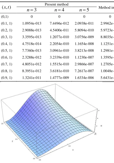
n , n4are shown in Table I. The numerical solutions for n3 and the exact solution are shown in Fig. 1 and Fig. 2.
Table I.
THE ABSOLUTE ERRORS FOR DIFFERENT
n
( , )x t Present method Method in [21]
3
n n4 n5
(0,1) 0 0 0 0
[image:4.595.280.553.51.284.2](0.1, 1) 1.0954e-013 7.4496e-012 2.0938e-011 2.9962e-005 (0.2, 1) 2.9088e-013 4.5400e-011 5.8094e-010 5.9723e-005 (0.3, 1) 3.3595e-013 1.2077e-010 3.0756e-009 8.8035e-005 (0.4, 1) 4.7518e-014 2.2054e-010 1.1654e-008 1.1251e-004 (0.5, 1) 7.7360e-013 3.0961e-010 3.8213e-008 1.2981e-004 (0.6, 1) 2.3288e-012 3.2339e-010 1.1230e-007 1.3595e-004 (0.7, 1) 4.8051e-012 1.5515e-010 2.9866e-007 1.2705e-004 (0.8, 1) 8.3951e-012 3.6181e-010 7.2617e-007 1.0048e-004 (0.9, 1) 1.3241e-011 1.4777e-009 1.6334e-006 5.6431e-005
Fig.1. The numerical solutions forn3.
In Table I, we list the results obtained by the Legendre polynomials method proposed in this paper together with the finite difference method [21] results. The displayed results show that our method is more convenient and more accurate
IAENG International Journal of Applied Mathematics, 47:3, IJAM_47_3_07
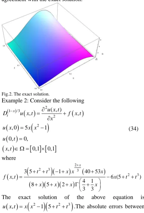
[image:4.595.303.542.381.723.2]than the finite difference method. From Fig. 1 and Fig. 2, we can see clearly that the numerical solutions are very good agreement with the exact solution.
Fig.2. The exact solution.
Example 2:Consider the following
2 1 /3
2 2
( , )
, ,
, 0 5 1
0, 0,
, 0,1 0,1
x t
u x t
D u x t f x t
x
u x x x
u t
x t
(34)
where
2
2 3 3
2 3
3 5 1 40 53
, 6 (5 )
4 1 8 5 2
3 3
x
t t x x x
f x t x t t
x x x x
The exact solution of the above equation is
2
2 3
, 1 5
u x t x x t t .The absolute errors between the exact solution and the numerical solution are displayed as follows:
Fig. 3. The absolute error for Example 2 of n3.
From Fig. 3, we can find that the absolute errors are very tiny and only a small number of Legendre polynomials are needed whenn3.
VI. CONCLUSION
In this paper, we have proposed a numerical approach for solving the variable order time fractional diffusion equation by using Legendre operational matrix. The operational
matrix of differentiation
D
andD
q x t( , )have been used for transforming the variable order time fractional diffusion equation into a Sylvester equation that can be solved easily. Finally, numerical example reveals that the present methodis very accurate and convenient for solving this problem.
REFERENCES
[1] Y.L. Li and W.W. Zhao, ―Haar wavelet operational matrix of fractional order integration and its applications in solving the fractional order differential equations,‖ Appl. Math. Comput., vol.216, pp. 2276-2285, 2010.
[2] H. Song, M.X. Yi, J. Huang, Y.L. Pan, ―Numerical solution of fractional partial differential equations by using Legendre wavelets,‖
Engineering Letter, vol.24, no.3, pp. 358-364, 2016.
[3] Z.M. Yan, F.X. Lu, ―Existence of a new class of impulsive Riemann-Liouville fractional partial neutral functional differential equations with infinite delay,‖ IAENG International Journal of Applied Mathematics, vol. 45, no. 4, pp.300-312, 2015.
[4] M. Ichise, Y. Nagayanagi, T. Kojima, ―An analog simulation of noninteger order transfer functions for analysis of electrode process, ― Journal of Electroanalytical Chemistry, vol.33, pp. 253- 265, 1971. [5] H.H. Sun, A.A. Abdlwahad, B. Onaral, ―Linear approximation of
transfer function with a pole of fractional order,‖ IEEE Transactions on Automatic Control, vol.29, pp. 441-444, 1984.
[6] O. Heaviside, Electromagnetic Theory, Chelsea, New York, 1971. [7] R.C. Koeller, ―Application of fractional calculus to the theory of
viscoelasticity,‖ Journal of Applied Mechanics,vol.51, pp. 299-307, 1984.
[8] H. Song, M.X. Yi, J. Huang, Y.L. Pan, ―Bernstein polynomials method for a class of generalized variable order fractional differential equations,‖ IAENG International Journal of Applied Mathematics, vol.46, no.4, pp. 437-444, 2016.
[9] W. Chen, ―A speculative study of 2/3-order fractional Laplacian modeling of turbulence: Some thoughts and conjectures,‖ Chaos, vol.16, 023126, 2006.
[10] Asgari M, ―Numerical Solution for Solving a System of Fractional Integro-differential Equations‖, IAENG International Journal of Applied Mathematics, vol. 45, no. 2, pp.85-91, 2015.
[11] S.G. Samko, B. Ross, ―Integration and differentiation to a variable fractional order,‖ Integral Trans. Special Func., vol.1, no.4, pp. 277- 300, 1993.
[12] S.G. Samko, ―Fractional integration and differentiation of variable order,‖ Anal. Math., vol.21, pp. 213-236, 1995.
[13] R.Lin, F. Liu, V. Anh, I. Turner, ―Stability and convergence of a new explicit finite-difference approximation for the variable-order nonlinear fractional diffusion equation,‖ Appl. Math. Comput., vol.212, pp. 435-445, 2009.
[14] P. Zhuang, F. Liu, V. Anh, I. Turner, ―Numerical methods for the variable-order fractional advection-diffusion equation with a nonlinear source term,‖ SIAM J. Numer. Anal., vol.47, pp. 1760- 1781, 2009. [15] C. Chen, F. Liu, V. Anh, I. Turner, ―Numerical schemes with high
spatial accuracy for a variable-order anomalous subdiffusion equation,‖ SIAM J. Sci. Comput. ,vol.34, no. 4, pp. 1740-1760, 2010. [16] A.Saadatmandi, ―A new operational matrix for solving fractional-order
differential equations,‖ Computers and Mathematics with Applications, vol. 59, pp. 1326-1336, 2010.
[17] S. Nemati and Y. Ordokhani, ―Legendre expansion methods for the numerical solution of nonlinear 2D Fredholm integral equations of the second kinds,‖ J. Appl. Math. Informatics, vol.31, pp. 609–621, 2013. [18] S. Abbasbandy, S. Kazem, M.S. Alhuthali, H.H. Alsulami,
―Application of the operational matrix of fractional-order Legendre functions for solving the time-fractional convection diffusion equation,‖ Appl. Math. Comput., vol.266, pp. 31-40, 2015.
[19] M.S. Islam, M.B. Hossain, ―Numerical solutions of eighth order BVP by the Galerkin residual technique with Bernstein and Legendre polynomials,‖ Appl. Math. Comput., vol.261, pp. 48-59, 2015. [20] C. F. M. Coimbra, ―Mechanics with variable-order differential
operators,‖ Ann. Phys., vol.12(11/12), pp. 692-703, 2003.
[21] S. Shen, F. Liu, J. Chen, et al., ―Numerical techniques for the variable order time fractional diffusion equation,‖ Applied Mathematics and Computation, vol.218, pp. 10861-10870, 2012.