Feedback Control for a Diffusive Delay Logistic
Equation: Semi-analytical Solutions
H.Y. Alfifi and T.R.Marchant
Abstract—Semi-analytical solutions are considered for a delay logistic equation with non-smooth feedback control, in a one dimensional reaction-diffusion domain. The feedback mecha-nism involves varying the population density in the boundary region, in response to the population density in the centre of the domain. The effect of the two sources of delay, from the logistic equation itself and the feedback term, is explored. The Galerkin method, which assumes a spatial structure for the solution, is used to approximate the governing partial differential equation by a system of ordinary differential equations. The form of feedback is chosen to leave the steady-state solution unchanged and guarantee positive population densities at the boundary. Whilst physically realistic, the feedback is non-smooth as it has discontinuous derivatives. A local stability analysis, of the four smooth parts of the full system, allows a band of parameter space, in which Hopf bifurcations occur, to be found. A precise estimate of the Hopf bifurcation parameter space, for the non-smooth system, is obtained using a hybrid stability condition. This is found by considering the dominant eigenvalues of the smooth parts of the system. Examples of bifurcation diagrams, stable solutions and limit cycles are shown in detail. Comparisons of the semi-analytical and numerical solutions show that the semi-analytical solutions are highly accurate.
Index Terms—logistic equation, reaction-diffusion-delay equations, non-smooth feedback control, Hopf bifurcations, semi-analytical solutions
I. INTRODUCTION
R
EACTION-diffusion equations with delays arise in many fields such as biology, chemistry, population ecology and physics, and have been investigated extensively. The introduction of a delay into the governing equation can introduce instability, via a Hopf bifurcation, with the sub-sequent development of limit cycles and periodic solutions. [1] introduced a delay into the competition term and obtained the delay logistic equationdu
dt =λu(t)(1−u(t−1)), (1) which has a steady-state solution for0< λ < π2 and periodic solutions for λ > π2, see [2]. [3] considered a generalised logistic equation with distributed delay. The form of the delay allowed the generalised delay equation to be written as a set of two coupled point delay equations. Explicit expressions were then obtained for the occurrence of Hopf bifurcations. [4] found an asymptotic solution to the delay logistic equa-tion, for the case when the delay is large. He derived explicit expressions describing the periodic solution, including the
Manuscript received June 2018
H.Y. Alfifi is with Department of Basic Sciences, College of Education, Imam Abdulrahman Bin Faisal University, Dammam, Saudi Arabia. email: [email protected].
T.R Marchant is with the School of Mathematics and Applied Statistics, The University of Wollongong, Wollongong, 2522, N.S.W., Australia. email: tim [email protected].
period and the maximum and minimum amplitudes. A good comparison was found between the analytical and numerical solutions, for large λ. [5] studied the stability of a model for pluripotent stem cell dynamics while [6] investigated the boundedness and stability of solutions to a Nicholson-type delay system. [7] considered classes of functional differential equation models which arise in attempts to describe temporal delays in HIV pathogenesis and [8] studied Nicholson-type systems with delays and considered the existence of positive periodic solutions.
The effects of feedback control in biology have been studied by many authors. [9], [10] considered feedback regulation of a logistic growth system, and considered the feedback delay. Sufficient conditions were obtained for the global asymptotic stability for the logistic equation in the delay feedback case. [11] experimentally considered the control of the collective dynamics with global time-delayed feedback in populations of electrochemical oscillators. Direct and differential delayed feedbacks were implemented. They also showed the effects of feedback gain and time delay on the collective behaviour of the populations.
Semi-analytical models of reaction-diffusion equations have been developed for a range of applications, such as the reversible Selkov model with feedback delay [13], the logistic equation [14] and the Brusselator model [15]. All these models yielded accurate solutions, compared with the full numerical results. [16] examined semi-analytical solu-tions for the Belousov-Zhabotinskii equasolu-tions in a reaction-diffusion cell. Non-smooth feedback control, with delay, was investigated. The Galerkin method was used to approximate the governing delay pdes by a system of delay odes. Steady state, transient solutions and Hopf bifurcation points were found. A band of parameter space was found, in which the Hopf bifurcations occur. Examples of a stable and unstable limit cycle were shown with an excellent comparison ob-tained between semi-analytical and numerical solutions.
[17] investigated bifurcation theory for non-smooth piece-wise continuous ode systems. Many important applications, such as control and switching problems, friction systems and impact oscillators, are described by such systems. They reviewed bifurcation theory for steady-state solutions which lie on discontinuity boundaries and described the new types of instabilities which can occur in the non-smooth system. [18] considered the stability of a plane piecewise smooth linear system with two dependent variables and discontinu-ous derivatives at the steady-state solution. They obtained a hybrid condition for the overall stability of the system, which related the complex eigenvalues of the two smooth systems, which comprised the full non-smooth system.
In this paper, we study the delay logistic equation in a 1-D reaction-diffusion cell with non-smooth feedback control. The feedback consists of varying the population density in
IAENG International Journal of Applied Mathematics, 48:3, IJAM_48_3_11
the boundary region in response to the population density in the domain centre. Also, to be physically realistic, the population density at the boundary must be positive, which requires the introduction of a modulus term in the feedback response, leading to a non-smooth system. Another key aspect of the problem is the effect of two different delay terms, on the stability of the system. The Galerkin method is used to find a semi-analytical model consisting of a set of non-smooth delay odes. The non-smooth system consists of four different sets of smooth odes, and we first study the stability of each smooth part of the system. This approach gives three regions, a region in which all smooth parts of the system are stable, a region in which all are unstable, and an intermediate region where some smooth parts are stable and some are unstable. The ideas of [16]–[18] are then used to provide a precise semi-analytical prediction of the region Hopf bifurcations occur for the full non-smooth system.
In Section II the semi-analytical ode model is derived using the Galerkin method for a 1-D cell geometry. In Section III a stability analysis is performed to determine the points of Hopf bifurcation with parameter maps of the Hopf points drawn. In Section IV steady state, limit cycle solutions and bifurcation diagrams are presented. Good comparisons are found between the semi-analytical and numerical solutions. In Section V some conclusions are made.
II. SEMI-ANALYTICAL MODEL
The diffusive delay logistic pde, for a 1-D geometry, is written as
ut=uxx+λu(t)(1−u(t−τ1)), (2) u(x, t) = 0, at x=±1, u(x, t) =ua, t≤0.(3) where u(x, t) represents the population density, λ is the growth or proliferation rate andτ1represents the delay term
in the logistic equation. The boundary condition (3) is of Dirichlet form with a zero population and the initial condition represents an uniform population ua for t ≤0. (2) and (3) has an unique steady-state solution and we letu=usbe the steady-state solution at the domain centre, x= 0. The pde (2) and (3) has oscillatory solutions; [14] mapped the areas of parameter space, in which Hopf bifurcations occurred.
One of the key aims of control is to change the stability of steady-state solutions via alteration of a parameter, in response to feedback from the system. For the pde (2) we use feedback of the form
u(x, t) =H|us−u(0, t−τ2)|, at x=±1, (4) at the boundaries. Now for a stable systemu(0, t)→usas t → ∞so the feedback does not change the occurrence of steady-state solutions.H >0is the feedback parameter and this response is proportional to the difference between the transient and steady-state solutions at x= 0. The modulus sign ensures that the population in the boundary region is always positive, as negative populations are unphysical. Note that the modulus term results in a continuous feedback system but with non-smooth derivatives. It is of interest here to determine how the feedback (4) modifies the stability of (2) and (3).
The Galerkin method is used for the derivation of a semi analytical model for (2) and (4). In this method, a spatial
form of the profile concentration is assumed, see [13], [14]. The Galerkin method is an analytical technique, which uses orthogonality of basis functions, so that we can replace the system of pdes by a lower order system of odes. In this model, the following trial function is used for the expansion
u(x, t) = (u1(t)−H|u1s+u2s−u1d2−u2d2|) cos
πx
2
+u2(t) cos 3πx
2
+H|u1s+u2s−u1d2−u2d2|, (5)
where uid2 =ui(t−τ2), i= 1,2.
The trial expansion (5) is chosen so thatu=u1+u2 is the
population density at the domain centre and the boundary condition (4) is satisfied. At the steady-stateus=us1+us2.
The pde (2) is not satisfied exactly, but the free parameters in the above expression are created from evaluating aver-aged versions of the governing pde, weighted by the basis functionscos 12πx
andcos 32πx
. Therefore, we obtain a system of two odes as
du1 dt =
2π
Hπ−4H+π[− π2
8 u1+λ( 1 2u1−
4
15πu2u1d1
− 36
35πu2u2d1−
4
3πu1u1d1) +λH(
4
3πu1M2− 1 2u1M2
−1
2u1d1M1+
4
15πu2d1M1+
4
3πu1d1M1+
4
15πu2M2)
+λHM1( kπ2
8 −
10
3πHM2+ 4−π
2π +HM2)
− 4
15πλu1u2d1], (6)
du2 dt =
6π 3π+ 4H[−
9kπ2
8 u2+λ( 1 2u2−
36 35πu2u1d1
+ 4
9πu2u2d1−
4
15πu1u1d1) +λH(
36 35πu2M2
−1
2u2M2− 1
2u2d1M1+
36
35πu2d1M1+
4
15πu1M2)
+λHM1( 2
5πHM2− 2 3π+
4
15πu1d1)−
36
35πu1u2d1λ],
M1=f(u1s+u2s−u1d2−u2d2),
M2=f(u1s+u2s−u1dd−u2dd), f(u) =sgn(u)u
uid1=ui(t−τ1), uid2 =ui(t−τ2),
uidd=ui(t−τ1−τ2) i= 1,2.
The series (5) is truncated after two terms, which represents a trade-off between the complexity of the expressions and the accuracy of the semi-analytical solution. Sufficient accuracy with little expression swell is provided by two-term method. The one-term solutions are derived by allowing u2 = 0.
As (6) includes modulus terms, it represents a non-smooth system with discontinuous derivatives. Depending on the sign of the two expressions involving the modulus signs (M1
andM2 in (6)) we have four different smooth ode systems,
termedpp,pn,npandnn, whereprefers to thesgnfunction inM1 or M2 being positive andn to it being negative.
In order to obtain the steady-state solutions, we let du1
dt = du2
dt = 0 in (6), which reduces them to sets of transcendental equations. We also note that at the steady state, the feedback response (involving the parameter H) terms can be neglected. The Maple software package is then used to obtain the steady-state solutions by solving the transcendental equations, h1 = h2 = 0. The
fourth-order Runge-Kutta scheme and the Crank-Nicholson finite
IAENG International Journal of Applied Mathematics, 48:3, IJAM_48_3_11
difference method are used to calculate numerical solutions to the ode and pde models, respectively. The temporal and spatial and temporal discretizations use for the finite-difference scheme are∆x= 0.05and∆t= 1×10⁻². This
implicit scheme is unconditionally stable.
III. STABILITY ANALYSIS AND BIFURCATION DIAGRAMS This section discusses the theoretical approach for the stability analysis, to determine the points of Hopf bifurcation. Stability theory is well understood for systems of smooth odes but it is less well developed for non-smooth ode systems, see [16]–[18] for a review of current theories. The analysis of the semi-analytical non-smooth ode system is a generalisation of [17], [18], who developed the stability of a non-smooth system consisting of two smooth linear ode systems. We explore the role the dominant eigenvalues of the smooth parts of (6) play, in the development of a hybrid stability condition. A semi-analytical map in which Hopf bifurcations occur is found and compared with numerical results. Also, the effects of the delay terms in the logistic pde and feedback are studied in detail. Hopf bifurcation points are studied for the delay ode model (6). The smooth ode systems are expanded in a Taylor series about the steady-state solution
ui=uis+gie−µt, i= 1,2, 1 (7) We substitute these expressions into the odes (6), and lin-earise around the steady state. µ is the growth rate and gi represent the amplitudes of the small perturbations at time t= 0. The Jacobian matrix gives the characteristic equation F(µ) =m1+im2= 0 for the decay rateµ. We setµ=iw
to be purely imaginary and the points of Hopf bifurcation then occur for
h1=h2=m1=m2= 0. (8)
The Hopf bifurcation curves, of the two smooth ode systems, pp andnn, are very similar to the two smooth systems,pn and np, respectively, with the curves the same to graphical accuracy. So, the two smooth systems ppandnnare found and plotted. This approach gives three regions: a region in which both smooth odes (pp and nn) of the system are stable; a region in which both are unstable; and a mixed region in which one ode is stable and the other unstable. Hopf bifurcations for the full non-smooth ode system occur in this mixed region of the parameter space.
To resolve the exact parameter space in which Hopf bifurcations occur for the non-smooth system (6), we first consider a linear non-smooth system, see [17].
˙
v=
A−v if cTv≤0,
A+v if cTv≥0, (9)
where the eigenvalues ofA± andλ=ς±±iω±, (ω±>0)
are complex, the steady state solution v = 0 and A± ∈ R2×2, c=R2. Then the discontinuous system (9) is stable
if
λs= ς +
ω+ + ς−
ω− <0. (10)
An insight into this combined stability condition can be found by letting the solutions
v=deς±tcos(ω±t), (11)
0 1 2 3 4 5
2 3 4 5 6 7 8
τ1
λ
pp smooth system
nn smooth system
numerical solution
(a)
0 1 2 3 4 5
2 3 4 5 6 7 8
τ1
λ
semi-analytical prediction
numerical solution
[image:3.595.307.535.61.414.2](b)
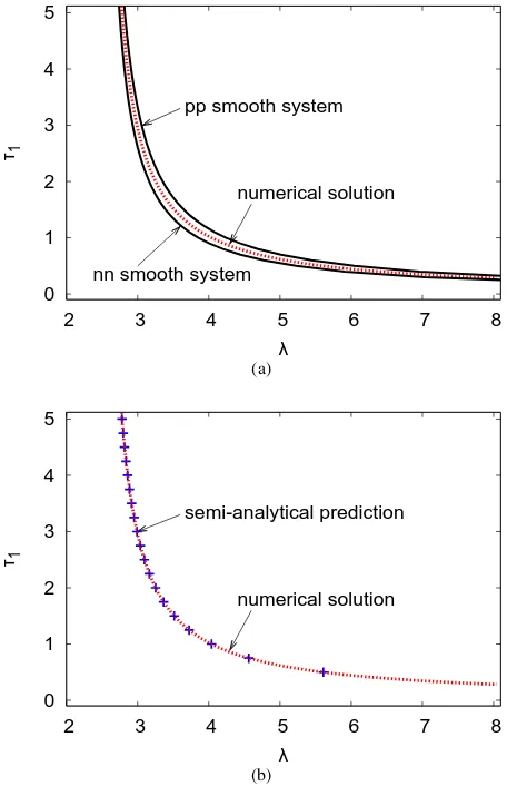
Fig. 1. (color online) Hopf bifurcation curves in theλ−τ1 plane with H= 0.1andτ2= 0. Shown are the two-term semi-analytical predictions (black solid line) of theppandnnsmooth systems, numerical solutions of (2) and (4) (red dotted line) and the semi-analytical prediction (10) for the non-smooth system-(blue crosses).
of the two odesv˙ =A±v. The solution stays in its portion of the phase plane space for timet= π
ω±, beforevchanges
sign. Hence, the growth or decay during this time is ςω±±π,
which leads to the combined stability condition (10). The two-term model (6) consists of two odes. In the parameter region where the Hopf bifurcation occurs the eigenvalues comprise a dominant complex conjugate pair plus other eigenvalues with negative real parts of larger magnitudes. Hence the dynamics of thepp and nnsmooth odes is governed by the dominant complex conjugate pair of eigenvalues and hence is similar to each smooth part of (9). If we assume that the components of the vectorv are all positive (theppcase where thesngterm forM1is positive)
att= 0, then at a later time the components will all become negative (thenncase where thesgnterm forM1is negative).
So if the dominant eigenvalues of the pp andnn cases are given by ς±±iω±, then (10) should apply with λs = 0
representing a condition for neutral stability. Hence we obtain a semi-analytical estimate of the parameter region in which Hopf bifurcations occur for the non-smooth system.
Figures 1 and 2 show Hopf bifurcation curves in theλ−τ1
plane with H = 0.1. The other parameters are τ2 = 0
and τ2 = τ1 respectively. Figures 1 and 2 (a) shows the
semi-analytical predictions from theppandnnsmooth ode
IAENG International Journal of Applied Mathematics, 48:3, IJAM_48_3_11
0 1 2 3 4 5
2 3 4 5 6 7 8
τ1
λ
numerical solution
pp smooth system
nn smooth system
(a)
0 1 2 3 4 5
2 3 4 5 6 7 8
τ
λ
semi-analytical prediction
numerical solution
[image:4.595.50.280.71.433.2](b)
Fig. 2. (color online) Hopf bifurcation curves in theλ−τ1 plane with H= 0.1andτ2=τ1. Shown are the two-term semi-analytical predictions (black solid line) of theppandnnsmooth systems, numerical solutions of (2) and (4) (red dotted line) and the semi-analytical prediction (10) for the non-smooth system-(blue crosses).
‘
0 1 2 3 4 5
2 3 4 5 6 7 8
τ1
λ τ2=3τ1 τ2=2τ1
τ2 = τ1
τ2=0
Fig. 3. (color online) Hopf bifurcation curves in theλ−τ1 plane with H= 0.1. Shown are the semi-analytical predictions (10) of the non-smooth system:τ2= 0(black dots),τ2=τ1 (blue dashed line),τ2= 2τ1(green solid line) andτ2= 3τ1(red dotted line).
systems, semi-analytical predictions (10) of the non-smooth system and numerical solutions. Figures 1 and 2 (b) show the numerical Hopf bifurcation points and the semi-analytical predictions (10) for the non-smooth system, for the same feedback cases. The stability curves for the sets of smooth odes separates the parameter space into three regions: one in which all smooth odes are unstable (the upper right part of the figure), one in which they are all stable (the lower left part of the figure); and third middle band of mixed stability. It can be seen that the numerical Hopf bifurcation points lie inside this mixed stability band. The semi-analytical predictions (10) for the non-smooth system lie inside this region of mixed stability and provide an accurate prediction of the numerical occurrence of limit cycles, with with errors less than1%for all choices ofλ.
Figure 3 shows Hopf bifurcation curves in the λ−τ1
plane withH = 0.1. Shown are the two-term semi-analytical predictions (10) for the non-smooth system for τ2 = 0, τ2=τ1,τ2= 2τ1andτ2= 3τ1. Asτ1increases, the critical
[image:4.595.51.280.525.722.2]value of the proliferation rateλis decreased for all cases, so feedback, from the more distant past, in the logistic equation itself is destabilizing. However, increasing the feedback delay has the opposite effect; for fixedτ1, increasing the value of τ2 stabilizes the system.
Figure 4 shows Hopf bifurcation curves in the λ−τ1
plane. Shown are semi-analytical predictions (10) of the non-smooth system for feedback with no delay, (a) τ2 = 0,
(b) τ2 = 0.5τ1, (c) τ2 = τ1. The feedback parameter H = 0,0.3,0.5 and 0.7. For all cases increasing the delay in the logistic equation, τ1, destabilizes the system and
the critical value of λ1 is decreased. The effect of the
feedback parameter H is to stabilize or destabilize regions of parameter space depending on the value of τ2. For the
case of feedback with no delay the system is destabilized asH increases, as the critical value of λis decreased asH increases. However, in the cases of feedback with delay, the effect of increasing the feedback parameterH is to stabilize the system, with the critical value ofλincreasing. Hence the interplay of feedback strength and delay is quite complex with both stabilizing and destabilizing scenarios possible.
Figure 5 shows Hopf bifurcation curves in the λ−τ2
plane. Shown are semi-analytical predictions (10) of the non-smooth system. The feedback parameter for four cases are H = 0.1,0.3,0.5 and 0.7 and τ1 = 2. Increasing the
delay in the feedback condition,τ2, causes the system to be
destabilized. However, the effect of increasing the feedback parameterH is stabilizing, so the combination of feedback together with delay can stabilize the system.
IV. BIFURCATION DIAGRAMS,STEADY-STATE AND TRANSIENT SOLUTIONS
In this section, bifurcation diagrams and the evolution to both steady-state solutions and limit cycles are considered. Note that the bifurcation diagram display long time solu-tions, of the steady-state amplitude and the maximum and minimum amplitudes of the periodic oscillations, so are not functions of the initial population ua. Also the bifurcation diagrams show the populations at the domain centre.
Figure 6 illustrates the steady-state profile for the popula-tion densityuversusx. The parameters are the proliferation
IAENG International Journal of Applied Mathematics, 48:3, IJAM_48_3_11
0 1 2 3 4 5
2.5 3 3.5 4 4.5
τ1
λ
H=0.7 H=0
H=0.3
H=0.5
(a) - Feedback without delay (τ2= 0)
0 1 2 3 4 5
2 3 4 5 6 7 8
τ1
λ
H=0
H=0.5 H=0.7
H=0.3
(b) - Feedback delay (τ2=12τ1)
0 1 2 3 4 5
2 3 4 5 6 7 8
τ1
λ
H=0
H=0.5 H=0.7
H=0.3
[image:5.595.308.535.73.234.2](c) - Feedback delay (τ2=τ1)
Fig. 4. (color online) Hopf bifurcation curves in theλ−τ1plane:H= 0
(black dots),H= 0.3(blue dashed line),H= 0.5(green solid line) and H= 0.7(red dotted line). Shown is the semi-analytical prediction (10) of the non-smooth system: (a) the caseτ2 = 0, (b) the caseτ2 = 12τ1, (c) the caseτ2=τ1.
0 1 2 3 4 5 6 7
2 3 4 5 6 7
τ2
λ
H=0
H=0.5 H=0.7
H=0.3
Fig. 5. (color online) Hopf bifurcation curves in theλ−τ2plane:H= 0.1
(black dots),H = 0.3(blue dashed line),H = 0.5(green solid line) and H= 0.7(red dotted line). Shown is the semi-analytical prediction (10) of the non-smooth system forτ1= 2.
0.2 0.4 0.6 0.8 1
0 5 10 15 20
u
λ
one-term two-term
[image:5.595.50.279.102.666.2]numerical solution
Fig. 6. (color online) The steady-state population densityuagainstx. The parameterλ= 10. Shown are the one-term (blue dashed line) and two-term (black solid line) semi-analytical solutions and the numerical solutions (red dotted line) of the pde (2).
0 0.2 0.4 0.6 0.8 1
-1 -0.5 0 0.5 1
u
x
one-term
numerical solution
two-term
Fig. 7. (color online) The steady-state population density u, against proliferation rateλatx= 0. Shown are the one-term (blue dashed line) and two-term (black solid line) semi-analytical solutions and the numerical solutions (red dotted line) of the pde (2).
IAENG International Journal of Applied Mathematics, 48:3, IJAM_48_3_11
[image:5.595.309.536.319.480.2] [image:5.595.311.536.564.728.2]0 1 2 3 4 5 6
2.5 3 3.5 4
u
λ
[image:6.595.310.540.58.221.2]two-term numerical solution
Fig. 8. (color online) Bifurcation diagram of the population densityufor H= 0.1andτ1=τ2= 2. The two-term (black solid line) semi-analytical solutions and numerical solution (red dotted line) are shown.
rate λ = 10 and τ1 = 0. Both one- and two-term
[image:6.595.52.282.59.222.2]semi-analytical of equations as well as numerical solutions of (2) and (3) are shown. The solution for the population density uhas a single central peak. A good comparison between the two-term semi-analytical and numerical solutions is obtained with an error of less than 1%. In this figure, the two-term case has a density of u= 0.85 atx= 0, very close to the numerical density, of u = 0.86. The one-term solution is reasonably accurate but does not model the flat population density profile, near the centre of the domain, accurately. The one-term density isu= 0.89atx= 0, an error of about3%. The accuracy of the semi-analytical profiles are qualitatively similar to those for cubic auto-catalytic reactions [19] and the Nicholson’s blowflies equation [14].
Figure 7 shows the steady-state population density u, versus proliferation rate λ. The one- and two-term semi-analytical models as well as numerical solutions are shown at x= 0. A unique steady-state solution for the population density u is found. The non-uniform steady-state solution bifurcates from the uniform steady-state solution u = 0
at λ = π42 and increases exponentially as λ increases, before approaching a maximum population density ofu'1. There is an excellent comparison between the two-term semi-analytical and numerical solutions, with no more than 2%
error for all values of proliferation rate up to λ= 20. Note that the numerical steady-state solution of (2) is found with the delayτ1= 0 as no Hopf bifurcations occur in this case.
Figure 8 shows the bifurcation diagram of the population densityu, forH = 0.1andτ1=τ2= 2. The numerical and
two-term semi-analytical solutions are obtained. The uniform steady-state solution,u= 0, occurs whenλ < π42. The non-uniform steady-state solution is stable for π42 < λ < λc. After the supercritical Hopf bifurcation point, λ > λc, periodic solutions occur. The two-term semi-analytical and numerical Hopf bifurcation points are λc = 3.31 and
3.32, respectively. The two-term semi-analytical solutions are extremely accurate in both the stable and oscillatory regimes of the bifurcation diagram. The main difference is a slight variation in the maximum amplitude of the oscillatory solution, for large λ, but is no greater than 4%, for the parameter ranges shown in this figure.
Figure 9 shows the bifurcation diagram of the population
0 1 2 3 4 5 6
2.5 3 3.5 4 4.5
u
λ
H=0.1
H=0
[image:6.595.309.535.283.443.2]H=0.3
Fig. 9. (color online) Bifurcation diagram of the population densityufor τ1 =τ2 = 2and H = 0(black solid line), H = 0.1(red dotted line) andH = 0.3(blue dashed line). The two-term semi-analytical solutions are shown.
0 1 2 3 4 5 6 7
2.5 3 3.5 4 4.5 5 5.5
u
λ τ2=2
τ2=3
τ2=1
Fig. 10. (color online) Bifurcation diagram of the population densityu forτ1= 2,H= 0.1andτ2= 1(blue dashed line),τ2= 2(black solid line) andτ2 = 3(red dotted line). The two-term semi-analytical solutions are shown.
density u for H = 0, 0.1 and 0.3. The other parameters are τ1 =τ2 = 2. The two-term semi-analytical is obtained
in each case. The two-term solutions lose stability at the supercritical Hopf bifurcation point, which occurs at λ = 3.25for the case with no feedbackH = 0andλ= 3.31,3.70
for the cases with feedback strength H = 0.1 and H = 0.3, respectively. It can be seen that the effect of increasing feedback strength is to stabilize the system. For the cases H = 0 and 0.1 the subcritical Hopf bifurcation point only moves slightly but the feedback causes a significant increase in the amplitude of the limit cycles, for larger values ofλ.
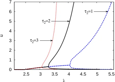
Figure 10 shows the bifurcation diagram of the population densityuforτ2= 1,2and3. The other parameters areτ1= 2 and H = 0.1. The two-term semi-analytical is obtained in each case. The two-term solutions lose stability at the supercritical Hopf bifurcation point, which occurs at λ = 4.06 for the case τ2 = 1 and λ = 3.31,3.11 for the cases τ2 = 2 and τ2 = 3, respectively. It can be seen that the
effect of increasing the delay parameter τ2 is to destabilize
the system, as the critical vale ofλis decreased.
Figures 11 shows the population density u, versus time t, at x = 0. The parameters are H = 0.1, ua = 0.1 and τ1 =τ2 = 2. Figure 11(a) has λ= 3.1 while figure 11(b)
IAENG International Journal of Applied Mathematics, 48:3, IJAM_48_3_11
0.1 0.2 0.3 0.4 0.5
0 10 20 30 40 50
u
t
numerical solution
two-term
(a) -λ= 3.1
0 0.2 0.4 0.6 0.8 1 1.2 1.4
0 10 20 30 40 50
u
t two-term
numerical solution
[image:7.595.50.281.57.415.2](b) -λ= 3.5
Fig. 11. (color online) The population densityuagainst timet, at point x= 0have the parametersH = 0.1,ua = 0.1andτ1 =τ2= 2. The
two-term semi analytical solutions are represented by black solid line while red dotted line represents numerical solutions.
has λ = 3.5. The two-term semi-analytical and numerical solutions are shown. For figure 11(a) λ= 3.1< λc = 3.31
and the solution evolves to a steady-state, withu(0, t)'0.25
as the time becomes large, after some initial relaxation os-cillations. There is an excellent comparison existing between the numerical and the two-term semi-analytical solutions, with an error not going beyond2%atλ= 50. The relaxation oscillations are also well modelled by the semi-analytical solution. For figure 11(b)λ= 3.5> λc= 3.31and periodic solutions occur. The numerical period and amplitude of the limit cycle are 6.86 and 1.25, respectively. These values are very close to the two-term semi-analytical period and amplitude, 6.87 and 1.26, respectively. The errors in the two-term semi-analytical values are less than 1%. Also the locations of the peaks and troughs of the limit cycle is well modeled by the semi-analytical solutions.
V. CONCLUSIONS
This paper has developed a lower-order semi-analytical model for the delay logistic equation with feedback control in the 1-D domain. The Galerkin method was used to obtain a system of delay odes. Steady-state solutions, limit cycles and Hopf bifurcation points were all found. Theoretical predictions for the Hopf bifurcation points were developed by examining the dominant eigenvalues associated with the
smooth parts of the ode system in order to obtain a hybrid stability condition for the non-smooth ode model. The effects of logistic equation and feedback delay were both considered, with both stabilizing and destabilizing scenarios possible. Comparisons of the two-term semi-analytical and numerical solutions further showed the utility of the semi-analytical method. Generally, the semi-analytical solutions represent a novel way of predicting the stability of non-smooth pde systems and future work will apply these methods to other relevant applications.
REFERENCES
[1] G. E. Hutchinson, “Circular causal systems in ecology,”Ann. New York Acad. Sci., vol. 50, pp. 221–246, 1948.
[2] T. Erneux,Applied Delay Differential Equations. New York: Springer, 2009.
[3] H. Rasmussen, G. C. Wake, and J. Donaldson, “Analysis of class of distributed delay logistic differential equations,” Math. Comput. Model., vol. 38, pp. 123–132, 2003.
[4] A. C. Fowler, “An asymptotic analysis of the delayed logistic equation when the delay is large,”J. Appl. Math., vol. 28, pp. 41–49, 1982. [5] M. Adimy, F. Crauste, and S. Ruan, “Stability and Hopf bifurcation
in a mathematicalmodel of pluripotent stem cell dynamics,”Nonlinear Anal-Real., vol. 6, pp. 651–670, 2005.
[6] C. Xu and M. Liao, “Boundedness and exponential stability of positive solutions for Nicholson-type delay system,” IAENG Inter. J. Appl. Math., vol. 45(2), pp. 151–157, 2016.
[7] H. T. Banks, D. M. Bortz, and S. E. Holte, “Incorporation of variability into the modeling of viral delays in HIV infection dynamics,”J. Math. Biol., vol. 183, pp. 63–91, 2003.
[8] L. Wang, P. Xie, and M. Hu, “Periodic Solutions in Shifts Delta(+/-) for a Nabla Dynamic System of Nicholson’s Blowflies on Time Scales”,IAENG Inter. J. Appl. Math., vol. 47(4), pp. 477–438, 2017. [9] K. Gopalsamy and P. Weng, “Feedback regulation of logistic growth,”
Internat. J. Math.&Math. Sci., vol. 16, pp. 177–192, 1993. [10] W. Wendi and T. Chunlei, “Dynamics of a delayed population model
with feedback control,” J. Austral. Math. Soc. Ser. B, vol. 41, pp. 451–457, 2000.
[11] Y. Zhai, I. Kiss, and J. Hudson, “Control of complex dynamics with time-delayed feedback in populations of chemical oscillators: Desynchronization and clustering,”Ind. Eng. Chem. Res., vol. 47, pp. 3502–3514, 2008.
[12] I. Huang, “Population dynamics viewed in feedback control,”Int. J. Control, vol. 18, pp. 563–569, 1973.
[13] K. S. Al Noufaey and T. R. Marchant, “Semi-analytical solutions for the reversible Selkov model with feedback delay,” Appl. Math. Comput., vol. 232, pp. 49–59, 2014.
[14] H. Y. Alfifi, T. R. Marchant, and M. I. Nelson, “Generalised diffusive delay logistic equations: semi-analytical solutions,”Dynam. Cont. Dis. Ser. B, vol. 19, pp. 5160–5173, 2012.
[15] H. Y. Alfifi, “Semi-analytical solutions for the Brusselator reaction-diffusion model.”ANZIM J., vol. 59, pp. 167–182, 2017.
[16] H. Y. Alfifi, T. R. Marchant, and M. I. Nelson, “Non-smooth feedback control for Belousov-Zhabotinskii reaction-diffusion equations: semi-analytical solutions.”J. Math Chem., vol. 57, pp. 157–178, 2016. [17] M. di Bernardo, C. Budd, A. R. Champneys, and P. Kowalczyk,
Piecewise-Smooth Dynamical Systems: Theory and Applications. Springer: London, 2008.
[18] M. K. Camlibel, W. Heemels, and J. M. Schumacher, “Stability and controllability of planar linear bimodal complementarity systems,” in Proceedings of the 42nd IEEE Conference on decision and control, Hawaii, USA, December 2003, pp. 1651–1656.
[19] T. R. Marchant, “Cubic autocatalytic reaction-diffusion equations: semi-analytical solutions,”Proc. R. Soc. Lond. A, vol. 458, pp. 873– 888, 2002.